Small Vision Transformers: A Tiny Diffusion Model on CIFAR-10
A 9.8 M parameter Diffusion Transformer learns to draw CIFAR-10 images in 86 minutes on one GPU. The loss is flat long before the samples look right.

On this page
The earlier posts in this series used a ViT to classify images. This post uses one to make images. A Diffusion Transformer (DiT) is a ViT that removes noise from an image. A model that can remove a little noise at a time can start from pure noise and end with a picture.
I trained a small DiT on CIFAR-10 and saved its samples every 5 epochs to see how they improve. The code is in the repo.
How a diffusion model works
A diffusion model learns to undo a simple process: adding noise to an image a little at a time.
Adding noise. Take a training image , with its pixel values scaled to the range from -1 to 1. Pick a step between 0 and 999. The noisy image at step is a mix of the image and random Gaussian noise :
The schedule fixes the two weights and for each step. At step 0, the image is almost clean. As grows, the image weight shrinks and the noise weight grows, until step 999 is almost pure noise. The figure below applies this to one CIFAR-10 image with the schedule that I use. The image is hard to see by step 175, even though its weight is still 0.85. The noise has a much larger effect than the weights suggest, because it changes every pixel independently.

Training. In each training step, the script takes a batch of images, picks a random step for each image, and adds noise as above. The model sees the noisy image and the step number, and it must predict the noise that was added. The loss is the mean squared error between the true noise and the predicted noise. This is the DDPM method (Ho et al., 2020).
Sampling. To make a new image, the model starts from pure noise at step 999. It predicts the noise, and from that prediction it can estimate what the clean image looks like. It then moves a little toward that estimate and repeats the process at a lower step. After enough steps, only the image is left.
The model
The model is a class-conditional DiT (Peebles and Xie, 2023). “Class-conditional” means that I tell it which class to draw. It has a patch size of 2, so a 32×32 image becomes 16×16 = 256 tokens. It has a width of 256, a depth of 8 and 4 heads, for a total of 9.8 M parameters.
The DiT looks like the classifier ViT from the first post, with three differences:
- It uses smaller patches. The classifier used patch size 4. A DiT must predict the noise for every single pixel, so it needs finer detail.
- It has no CLS token. The model does not output one class. Instead, each token outputs the predicted noise for its own 2×2 pixels and 3 colors, and the model puts these pieces back together into a 32×32 noise image.
- It takes two extra inputs. The model must know how noisy its input is (the step ) and what to draw (the class label). It turns each one into a vector of 256 numbers and adds the two vectors together into one condition vector.
The condition controls every block through adaptive layer norm (adaLN). A normal transformer block uses layer normalization, which rescales each token to a standard range. In a DiT, each block computes a shift and a scale for this normalization from the condition vector. It also computes a gate, a number that multiplies the block’s output before the model adds it back to the shortcut path. So the noise level and the class change how every block behaves.
The gates start at zero. Each block’s output is multiplied by zero at the start of training, so each block passes its input through unchanged. The paper calls this adaLN-Zero. The network starts as a simple, stable function and learns how much each block should add.
Training and sampling settings
- Class dropout: for 10% of the training images, the label is replaced by a special “no class” label. One model then learns two predictions: the noise for a given class, and the noise for any image at all.
- Classifier-free guidance: when sampling, the model makes both predictions at each step. The sampler then pushes the result away from the “any image” prediction and toward the class prediction: it takes the “any image” prediction and adds 2 times the difference between the two. The scale of 2 makes each sample look more like its class, but it also makes the samples less varied.
- DDIM sampling (Song et al., 2021): instead of 1,000 small steps, the sampler takes 100 larger steps. DDIM also adds no new randomness during sampling, so the same starting noise always gives the same image. I use this to compare snapshots from different epochs.
- EMA: the samples come from an exponential moving average (EMA) of the weights. After every training step, the averaged weights move 0.01% of the way toward the current weights (a decay of 0.9999). This smooths out the noise from single training steps.
- Optimizer: the model trains with AdamW at learning rate 3e-4, with no weight decay, a 1,000-step warmup and then a constant rate. Training runs for 200 epochs with batch size 128, horizontal flips and bfloat16 mixed precision.
The full run took 86.5 minutes on an RTX 3080 Ti, which is 26 seconds per epoch. The peak VRAM was 3,595 MiB.
The samples
Each row is one class, in CIFAR-10 order: airplane, automobile, bird, cat, deer, dog, frog, horse, ship, truck.
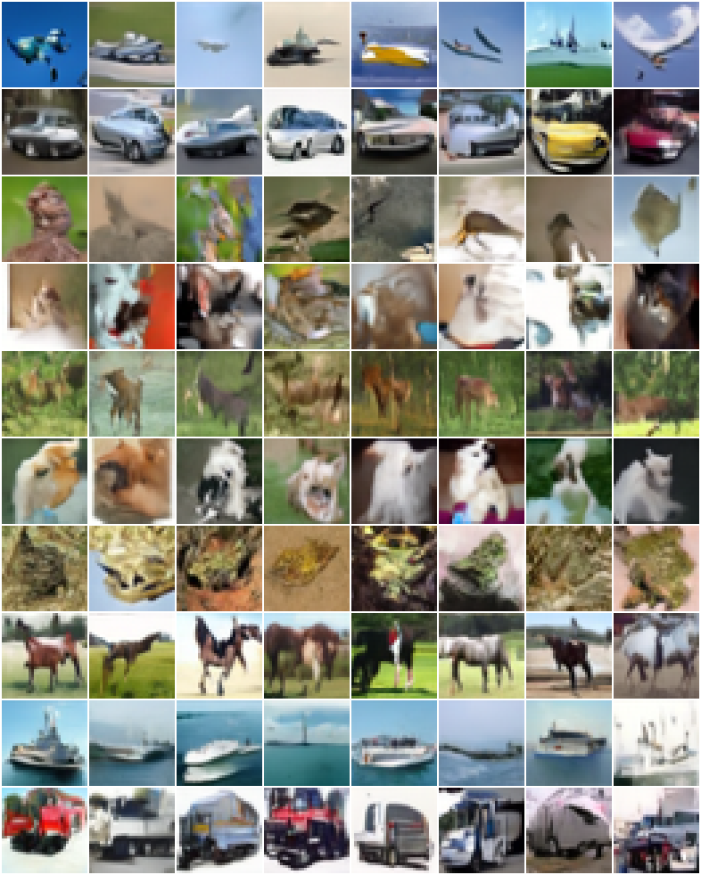
Airplanes, cars, horses, ships and trucks have clear shapes and plausible backgrounds. Cats, dogs, birds and frogs often have the right colors and texture, but a blurred or broken shape.
I measured FID (Fréchet Inception Distance, a standard score that compares generated images with real ones) for this model in the next post. On 10,000 samples, it’s 19.9 with 128 DDIM steps and 22.1 with 64 steps. I didn’t measure the 100 steps used for these samples.
The loss is flat, but the samples are not
The training loss drops fast and then almost stops: it is 0.033 at epoch 25 and 0.030 at epoch 200.
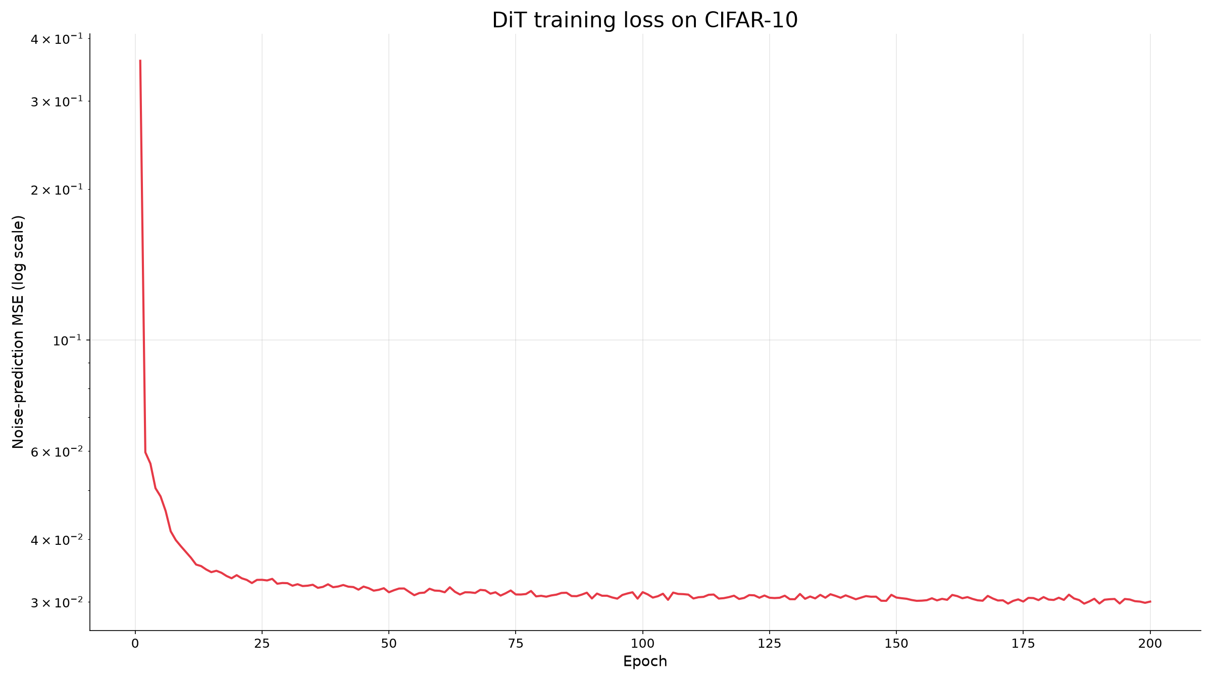
The samples tell a different story. The figure below starts from the same noise at six points during training.
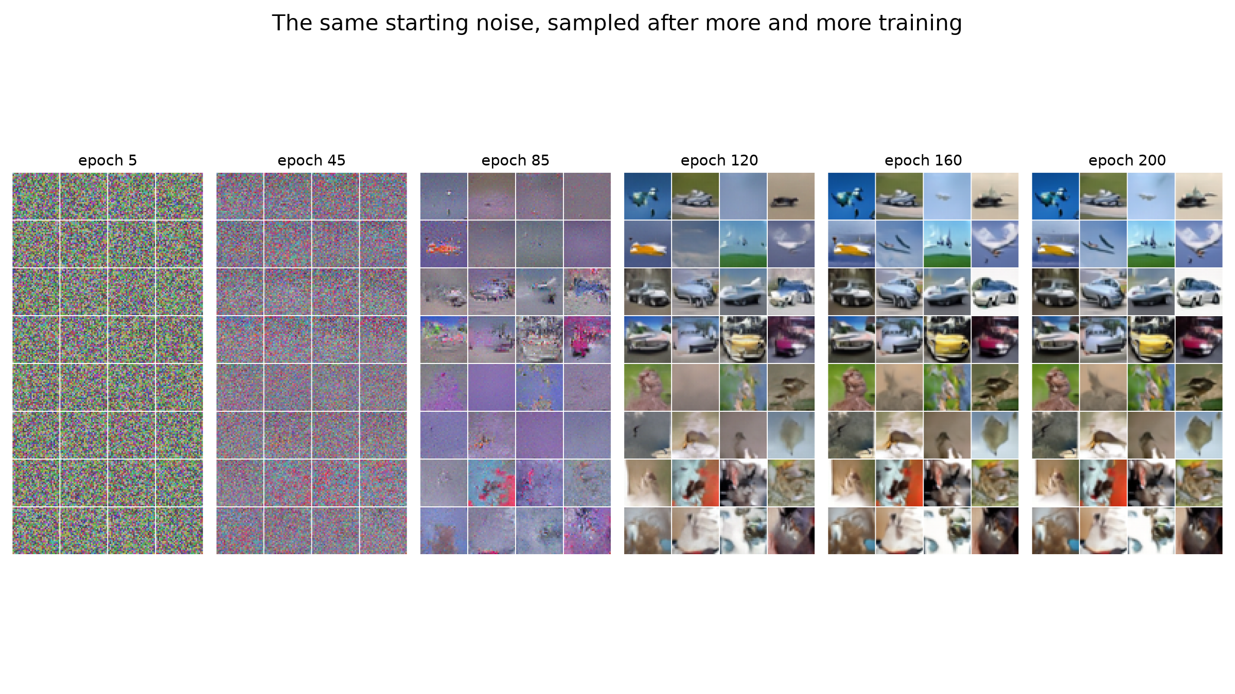
- At epoch 45, the samples are still noise.
- By epoch 85, objects appear.
- After epoch 120, the samples change little.
Part of the delay comes from the EMA. With a decay of 0.9999, the averaged weights trail the current weights by about 10,000 steps. One epoch is 391 steps, so the lag is about 26 epochs.
The loss is an average over all 1,000 noise levels, and I think this explains the rest. At most noise levels, the model can make a reasonable guess early in training. The details that make a sample look like a real object change this average only a little. So the loss alone would not have told me when the samples became good.
From noise to image
The next figure shows four sampling runs. At each of 10 points during sampling, it shows the clean image that the model predicts at that moment.
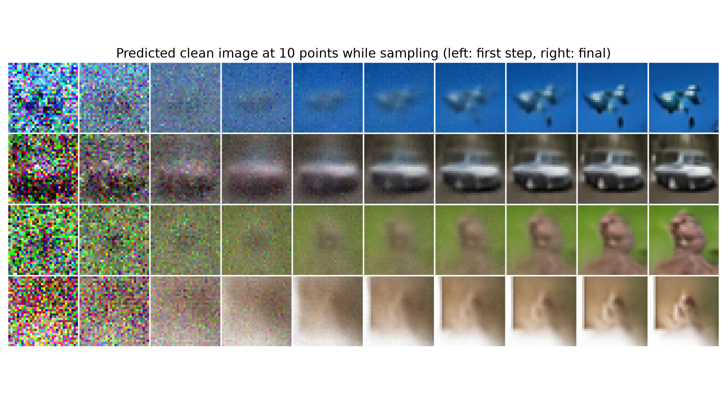
In these four rows, the background color and the rough layout appear first. The edges and the details come in the last steps. This order makes sense. At high noise levels, only large areas of color survive the noise, so that is all the model can predict. Fine details become visible only when most of the noise is gone.
Does it copy the training set?
A small model on a small dataset could memorize images and return copies of them. As a check, I put 10 samples next to the training image that is closest to each one in pixel space, I measure closeness with the L2 distance: I square the difference at every pixel value, add them up and take the square root.
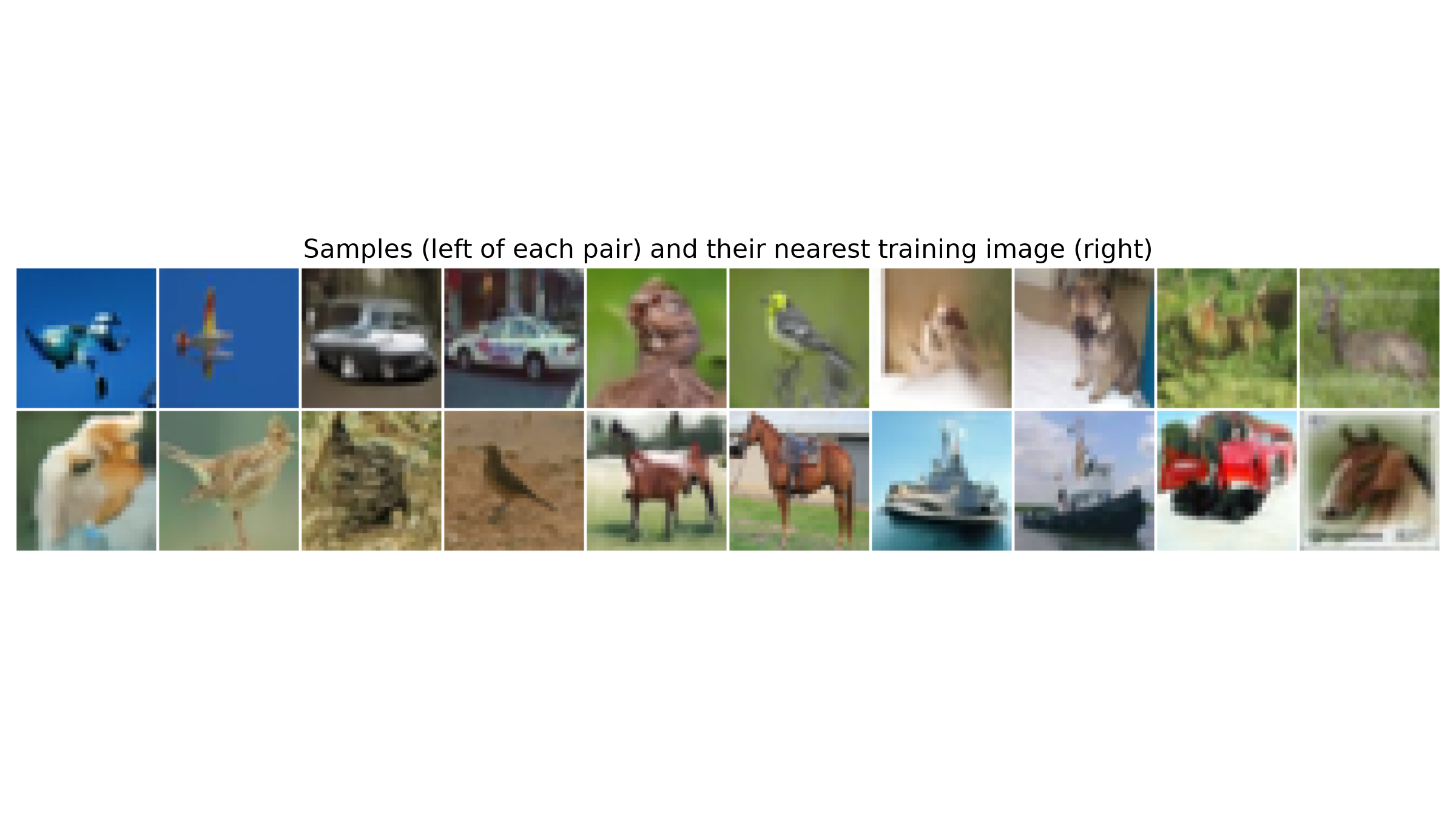
For all 10 samples, the nearest training image is a different image. The pairs share colors and layout, but they are not copies. This is a small check, not a proof.
What I take from this
- A diffusion model that draws recognizable objects fits in 9.8 M parameters and 86 minutes on one consumer GPU.
- Look at the samples, not only at the loss, to decide when a diffusion model is done.
- Remember the EMA lag. With a decay of 0.9999, the samples are about 26 epochs behind the weights.
I write about reinforcement learning, transformers, multi-agent systems, and the tools I build along the way.