Small Vision Transformers: Fine-Tune or Train from Scratch on 1,020 Images
ViT-B/16 on Flowers-102 with 10 images per class: 39.0% from scratch, 98.4% with a linear probe and 99.2% with LoRA, plus a check for leaked test images.

On this page
The first post showed that a ViT needs a lot of data when it starts from random weights. A ResNet has built-in habits, such as looking at nearby pixels first, and a ViT must learn them from its training images. Even with 50,000 images, the ViT stayed behind. This post asks the practical question: with a very small dataset, how much does a pretrained model help?
I took one dataset and one architecture, and I trained the model in three ways. The code is in the repo. All three runs together take about 10 minutes on an RTX 3080 Ti.
The dataset
Oxford Flowers-102 has photos of 102 flower species. The official training split has only 10 images for each class, which is 1,020 images in total. The test split has 6,149 images.
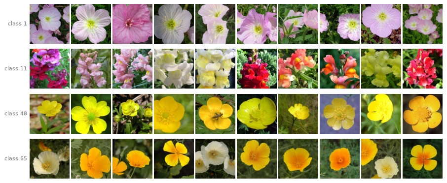
Ten images per class is very little. The figure below shows every training image for four of the classes. The photos differ in color, scale, background and number of flowers. Some classes also look alike: classes 48 and 65 are both yellow-to-orange flowers with round, open petals.
The model and its pretrained weights
The model is ViT-B/16. “B” stands for the Base size, with 12 layers, 12 attention heads per layer, a width of 768 and 86 M parameters. “16” is the patch size. The model takes 224×224 images, so it cuts each image into 14×14 = 196 patches of 16×16 pixels.
The pretrained weights are vit_base_patch16_224.augreg2_in21k_ft_in1k from the timm library. They come from a model that was first trained on ImageNet-21k, a set of about 14 million photos in about 21,000 classes, and then fine-tuned on ImageNet-1k, which has 1.3 million photos in 1,000 classes. This is the important part. During pretraining, the model already learned what the first post said a ViT must learn from data: which patches are neighbors, what edges and textures look like, and how parts form objects. It saw millions of photos to learn this. My task only has to teach it the differences between 102 flowers.
Three ways to train
| Method | Starting weights | Trainable parameters |
|---|---|---|
| From scratch | random | all |
| Linear probe | pretrained | the classifier head only |
| LoRA | pretrained | rank-8 LoRA on every qkv projection, plus the head |
From scratch starts every weight at a random value and trains all of them. The model sees only the 1,020 flower photos.
A linear probe keeps every pretrained weight frozen, which means that training does not change it. The pretrained model ends with a head, a last layer that turns the model’s output into scores for the 1,000 ImageNet classes. The probe throws that head away and puts a new one in its place, with random starting weights and one output for each of the 102 flower classes.
Here is what happens to one image:
- The frozen model reads the image through all 12 layers, exactly as it did after pretraining.
- After the last layer, the CLS token holds 768 numbers that summarize the image. These numbers are the image’s features.
- The new head computes one score for each flower class. Each score is a weighted sum of the 768 features plus a constant, called the bias. Each class has its own 768 weights and its own bias.
- The class with the highest score is the prediction.
The word “linear” refers to step 3. A weighted sum is the simplest kind of layer, and the head has no other layers in between. The head trains 768 × 102 weights plus 102 biases, which is 78 thousand numbers in total.
A probe can work this well only because of pretraining. The pretrained model already puts images that look alike close together in its 768-number feature space: two photos of the same species get similar features, and different species get different features. The head only has to learn where to draw the borders between the 102 groups. If the features did not separate the flowers well, no amount of training on the head would fix it. That is why people use a linear probe to measure how useful pretrained features are. The word “probe” comes from that use.
The probe is also cheap. Training changes only the head, so the gradients stop at the last layer and never travel back through the 12 frozen layers. The model still runs the frozen layers on every image in every epoch, because the augmentation gives a new crop each time.
LoRA (low-rank adaptation, Hu et al., 2021) also freezes the pretrained model, but it lets the attention layers change a little. In each layer, one weight matrix, called qkv, turns each 768-number token into its query, key and value, which are 2,304 numbers together. That matrix has 1.77 M weights. LoRA leaves it frozen and adds a small side path next to it:
- Matrix A squeezes the 768 input numbers down to 8.
- Matrix B expands those 8 numbers back to 2,304.
- The model adds the side path’s output to the output of the frozen matrix.
The number 8 is the rank. Because the side path goes through only 8 numbers, A and B together have 24,576 weights, which is 1.4% of the frozen matrix. Across the 12 layers, plus the new head, LoRA trains 373 thousand numbers.
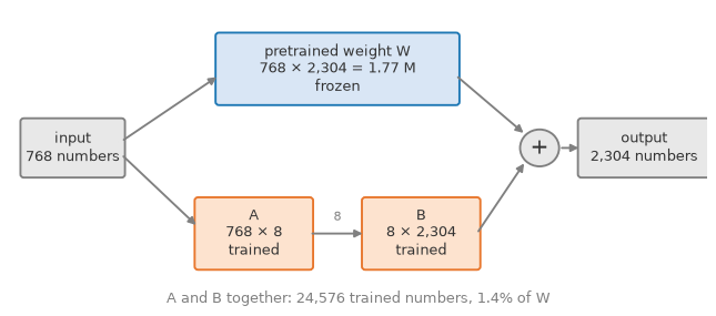
B starts at all zeros, so at the first step the side path adds nothing and the model behaves exactly like the pretrained one. Training then moves B and A away from that starting point. The side path’s output is multiplied by 2 (alpha 16 divided by rank 8), and it uses dropout of 0.1. You can check my LoRA implementation in the repo, here.
Training settings
All three methods use the same data, 30 epochs, batch size 32, and AdamW with 3 warmup epochs and cosine decay. Only the learning rate changes: 3e-4 from scratch, and 1e-3 for the probe and LoRA.
The augmentation is a random resized crop and a horizontal flip. The random resized crop cuts a random rectangle from the photo, with between 8% and 100% of the photo’s area, and resizes it to 224×224. So each epoch shows the model a different zoom and position of the same flower. At test time, the model sees one center crop instead.

Results
| Method | Test accuracy | Training time | Peak VRAM | Trainable parameters |
|---|---|---|---|---|
| From scratch | 39.0% | 2.7 min | 3,578 MiB | 85.9 M |
| Linear probe | 98.4% | 1.6 min | 513 MiB | 78 K |
| LoRA r=8 | 99.2% | 2.3 min | 2,112 MiB | 373 K |
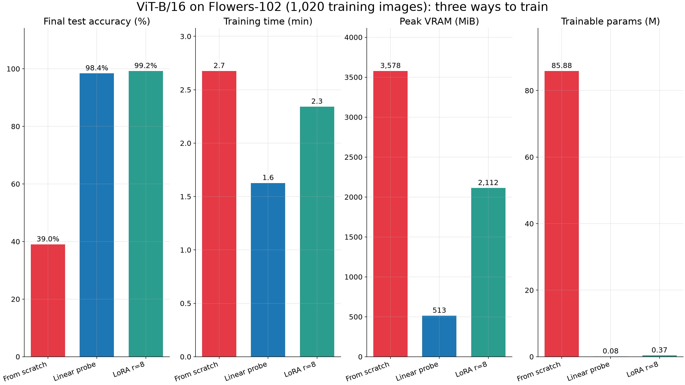
- Training from scratch does not work here. The model has 86 M parameters and only 1,020 images to learn from, and it reaches 39.0%. That is far better than random guessing (1%), but the model must learn everything about images from 10 photos per class.
- The linear probe gets 98.4%. It trains 78 thousand parameters in 1.6 minutes and uses 0.5 GB of VRAM. The pretrained features are already good enough that a single new layer separates 102 species.
- LoRA gets 99.2%. It trains 373 thousand parameters, which is 0.4% of the model. For the extra 0.8 points, it uses four times the VRAM of the probe, because training must send gradients back through every layer to reach A and B.
Each result is one run. I did not tune the hyperparameters on the test split, and the table shows the last epoch, not the best one.
Is 99% too good?
With a number like 99.2%, it is sensible to check the data. Maybe some test images also appear in the training split. So the repo has a check with three detectors, from strict to loose:
- Identical file bytes. The check computes a SHA-256 fingerprint of each file. Two files with the same fingerprint are exact copies.
- A perceptual hash (dHash). The check shrinks each image to a tiny grayscale thumbnail and compares each pixel with its neighbor, which gives 64 yes-or-no bits. Two photos that look the same give hashes that differ in only a few bits, even after resizing or recompression. The check also hashes the mirror image, so it catches flipped copies.
- Embedding similarity. The pretrained ViT-B/16 turns each image into a vector of 768 numbers, called an embedding. Cosine similarity measures how closely two of these vectors point in the same direction. A value of 1 means that the model sees the two images as the same. This detector catches crops and edits that the other two miss, but it also flags different photos of the same species.
The findings on the official split:
- Exact copies: 1 test image is byte-identical to a training image. In all 8,189 images, 4 pairs of files are byte-identical.
- Perceptual hash: 7 test images are within 6 bits of a training image. I reviewed them. Apart from the exact copy, they are different photos, and 4 of them are from different classes.
- Embeddings: 279 of the 6,149 test images (4.5%) have a cosine similarity of 0.95 or more to a training image, and 278 of these are in the same class. Many of the highest pairs are near-duplicates: the same flower in the same scene, photographed a moment apart. The others only show the same species.
The figure below shows the 12 test images with the highest similarity, each next to its closest training image. The first pair is the exact copy. Most of the other pairs show the same plant in the same scene, photographed again from a slightly different angle or distance.
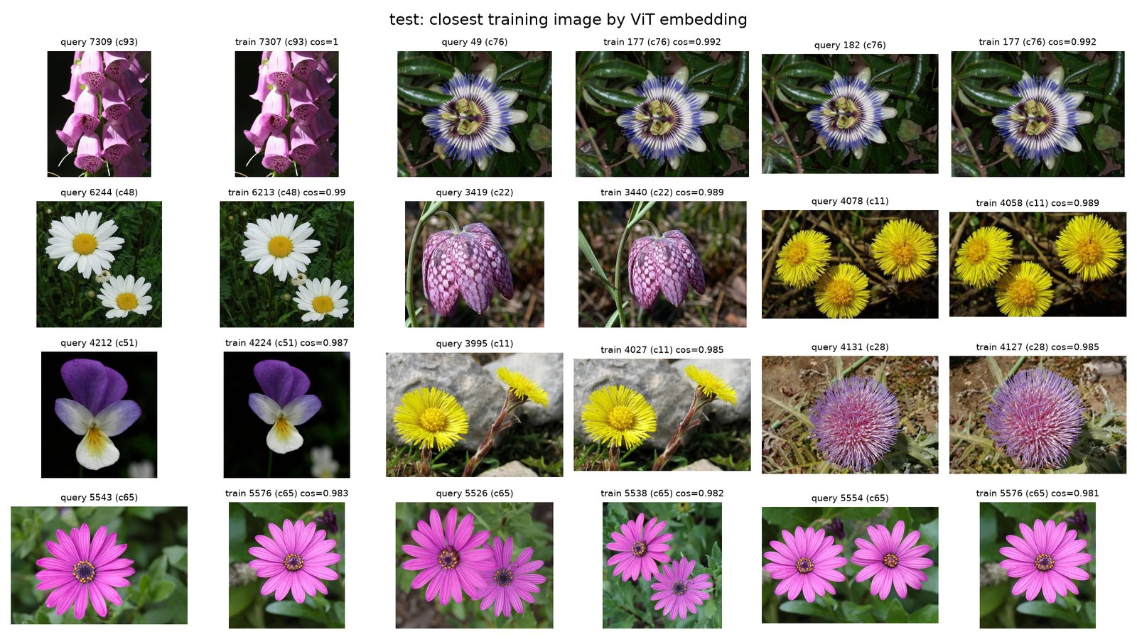
The near-duplicates are too few to change the conclusion. Take the worst case: remove all 279 flagged images and assume that the model got every one of them right. LoRA then drops from 99.2% to at least 99.1%, and the linear probe drops from 98.4% to at least 98.3%. For the model trained from scratch, the accuracy on the other 5,870 images is between 36.1% and 40.9%.
This check cannot answer one question: whether the test images are in ImageNet-21k, which the pretrained weights saw. I do not have that dataset here.
What I take from this
- With about 1,000 images, do not train a ViT-B/16 from scratch.
- Start with a linear probe. It is the cheapest method, and here it was only 0.8 points behind LoRA.
- Use LoRA when the last point of accuracy is worth the extra memory.
- When a result looks too good, check the split before you believe it.
The next post keeps the transformer but changes the job: a tiny diffusion model.
I write about reinforcement learning, transformers, multi-agent systems, and the tools I build along the way.