Small Vision Transformers: A ViT from Scratch on CIFAR-10, with the Failures
A small Vision Transformer starts at 57% on CIFAR-10 and reaches 92.9% after eight fixes. Each fix has a measured gain, and ResNet-18 still wins.

On this page
A Vision Transformer (ViT) divides an image into patches and treats them like the words of a sentence. It has no built-in understanding that nearby pixels belong together. A convolutional network has that idea from the start. The ViT must learn it from the data, and CIFAR-10 has only 50,000 training images.
So a small ViT that you train from scratch on CIFAR-10 is known to lose to a ResNet. In this post, I test this myself, and then I try to close the gap one fix at a time.
The code is in the repo. Every run in this post was trained on one RTX 3080 Ti.
The setup
CIFAR-10 is a set of 60,000 small color photos, each 32×32 pixels, in 10 classes such as airplane, cat, horse and truck. I train on the 50,000 training images and report the accuracy on the 10,000 test images.
The ViT has a width of 384, a depth of 7 and 6 attention heads. Width is the length of the vector that describes each patch, and depth is the number of transformer blocks. The model has 12.5 M parameters, close to the 11.2 M of ResNet-18.
- ViT optimizer: AdamW, learning rate 1e-3, weight decay 0.05, gradient clipping at 1.0.
- ResNet-18 optimizer: SGD with Nesterov momentum 0.9, learning rate 0.1, weight decay 5e-4.
- All runs: 100 epochs, batch size 512, cosine learning-rate decay, bfloat16 mixed precision.
Why a ResNet has a head start
A ResNet is a convolutional network. Each layer slides a small 3×3 filter, a tiny grid of learned weights, across the image. So each output pixel of the first layer depends only on one input pixel and its 8 neighbors. This design gives the network three useful habits before it sees a single training image.
- It looks locally first. A first-layer filter can only combine pixels that touch. Edges, corners and color spots are local patterns, so this is a good place to start.
- It reuses the same filter everywhere. The network applies one 3×3 filter at every position. If a filter learns to find a horse’s ear in one corner, it also finds an ear in the opposite corner. The network does not need training photos with a horse in every position.
- Its view grows layer by layer. Each stacked 3×3 layer widens the area that one output pixel sees. One layer sees 3×3 pixels, three layers see 7×7, and five layers see 11×11. Later layers also shrink the image by half, so by the last stage of ResNet-18, each output sees the whole 32×32 image. The network builds small parts into bigger ones: edges become textures, textures become an eye or a hoof, and those parts become a horse.
The ResNet does not learn these habits from data, because they come from its design. People call an assumption like this an inductive bias.
A ViT makes almost none of these assumptions. My ViT cuts the image into 4×4-pixel patches, so it gets 64 patches. It flattens each patch into 48 numbers (16 pixels × 3 colors) and maps them to a vector of 384 numbers called a token. In every block, attention lets each token take information from every other token, whether that token is near or far. Nothing in the math says that patch 27 sits next to patch 28.
The only clue about the layout is the position embedding. This is a learned vector that the model adds to each token, with one vector for each position. In my model, these vectors start as small random numbers. If you shuffle the patches together with their position vectors, the ViT gives exactly the same output. At the start of training, the position vectors carry no information, so the middle and right images below look the same to the model.
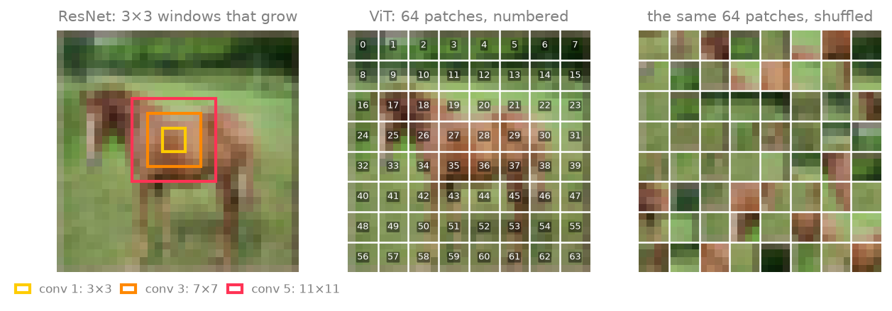
The ViT does have a little built-in structure. It uses the same patch-to-token mapping at every position, and the pixels inside a patch stay together. Everything above the patch level, such as which patches are neighbors and how parts form an object, it must learn from the training images. The next post shows that the trained ViT does learn this: some of its early attention heads focus on nearby patches, much like a convolution.
Learning this takes data. With only 50,000 images, the ViT starts far behind, and most of the fixes below either give it more varied data or make that learning easier.
The fixes
The ladder in the next section adds these changes one at a time. This section shows what each change does.
Random crop and horizontal flip
Data augmentation changes each training image a little every time the model sees it. The model sees a slightly different version of each photo in every epoch, so it is harder for it to memorize the training set.
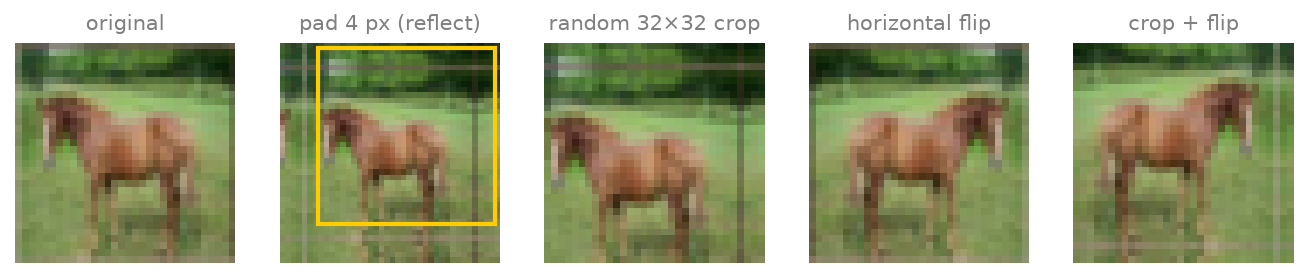
The first two changes are simple. The random crop adds a 4-pixel border around the image by mirroring its edges, and then it cuts a random 32×32 window from the result. This shifts the object by up to 4 pixels in any direction. The horizontal flip mirrors the image left to right half of the time. A horse that faces left is still a horse.
RandAugment
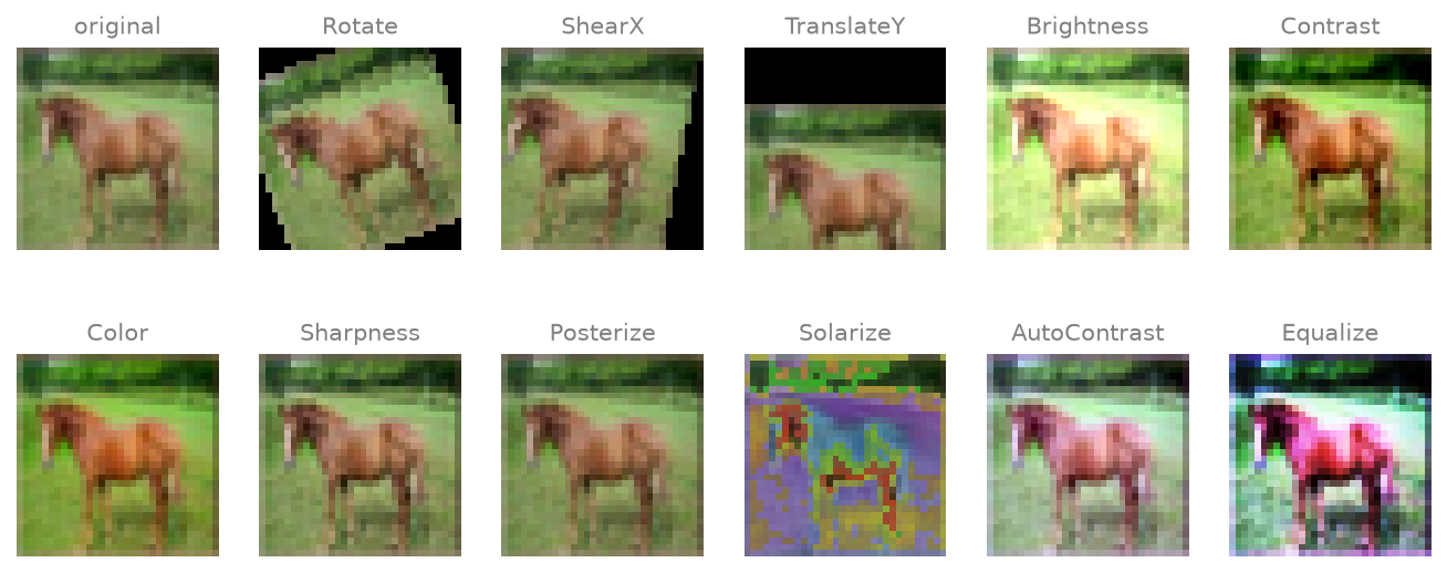
RandAugment (Cubuk et al., 2019) adds stronger changes. For each image, it picks 2 operations at random from a list of 14 and applies them at a fixed strength. The strength scale goes from 0 to 30, and I use 9. The operations fall into two groups:
- Geometry: rotate, shear (slant the image sideways), and translate (shift the image).
- Color and tone: brightness, contrast, color saturation, sharpness, posterize (use fewer color levels), solarize (invert the brightest pixels), auto-contrast and equalize (stretch the colors to use the full range).
The list also includes “identity”, which leaves the image unchanged. The figure below shows each operation on its own. I use strength 20 here instead of 9 so that the changes are easy to see. Even at strength 20, sharpness and posterize barely change a blurry 32×32 photo.
In training, the crop, the flip and RandAugment run together, with new random choices every time. These are eight versions of the same horse, as the model sees them in eight different epochs:

Smaller patches
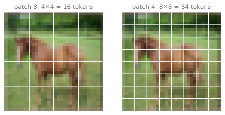
The first ViT uses 8×8-pixel patches, so it turns each image into 16 tokens. Patch size 4 gives 64 tokens. Each token now describes a smaller area, so small details such as a leg or an ear do not get averaged together into one token. The model also has four times as many tokens to compare with each other. The cost is compute: attention compares every token with every other token, so 4 times the tokens means about 16 times the attention work.
Learning-rate warmup
The learning rate sets the size of each weight update. With warmup, the learning rate starts near zero and rises in a straight line to its peak of 1e-3 over the first 10 epochs. After that, it follows the same cosine decay as before.
Warmup matters most at the start of training. The weights are random, and AdamW estimates the typical size of each gradient from only a few steps. So the first updates can be large and point in poor directions. In a transformer, a few large early updates can push the attention into a state where each token puts almost all of its weight on one other token. The model then learns very slowly. This is a common explanation, and it fits the stalled runs in the learning-rate study below.
Label smoothing
Normally, the training target for a horse photo says “100% horse”. With label smoothing at 0.1, the target says 91% horse and 1% for each of the other nine classes. The model is no longer pushed to be completely sure about every training image. This often helps when the model memorizes the training set.
MixUp and CutMix
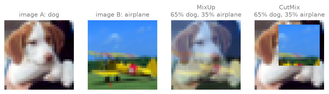
These two methods combine pairs of training images. For each batch, the code picks one of the two methods at random.
- MixUp (Zhang et al., 2018) blends two images pixel by pixel. If the blend is 65% dog and 35% airplane, then the target is also 65% dog and 35% airplane.
- CutMix (Yun et al., 2019) cuts a rectangle out of one image and pastes it into the other. The target follows the area: if the airplane covers 35% of the image, then the target is 35% airplane.
In training, the mix ratio and the rectangle position are random for each batch. The figure uses a fixed 65/35 split.
Stochastic depth
Stochastic depth (Huang et al., 2016) skips whole transformer blocks at random during training. Each block has a shortcut path around it, so a skipped block passes its input through unchanged. The chance of a skip rises from 0 in the first block to 10% in the last block. At test time, every block runs. The effect is similar to training many shallower networks that share their weights.
More epochs
The last step trains for 200 epochs instead of 100. Nothing else changes.
The training ladder
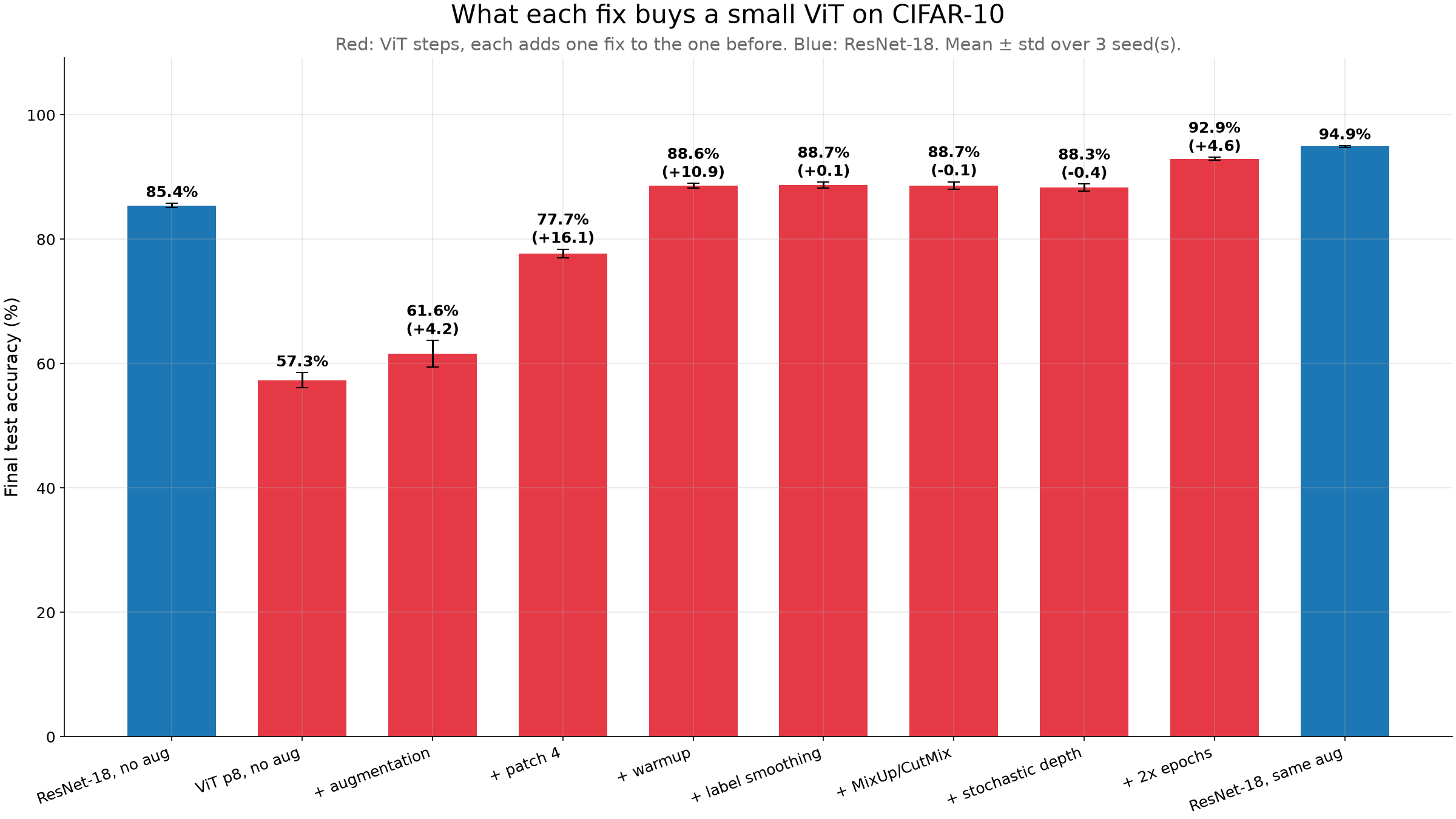
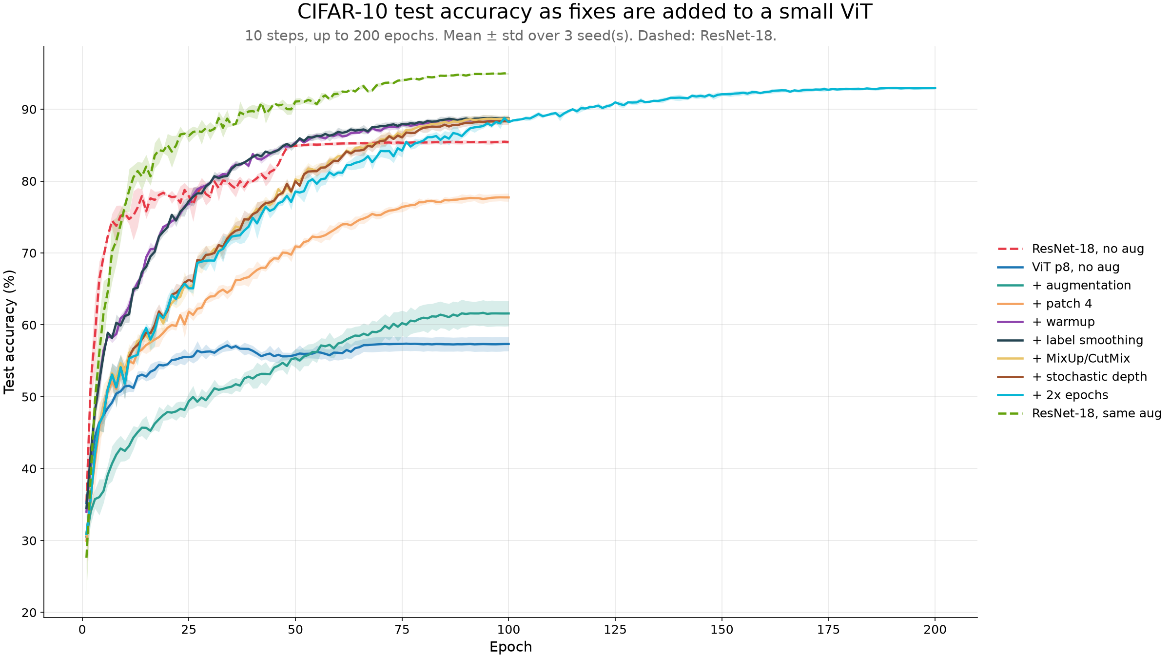
Each ViT step adds one change to the step before it. The difference between two neighboring steps is what that change buys. Every step ran with 3 seeds. The table shows the mean and the standard deviation of the test accuracy at the last epoch.
| Step | Change | Test accuracy | Gain | Time |
|---|---|---|---|---|
| ResNet-18 | no augmentation | 85.43 ± 0.34% | 10.6 min | |
| ViT | patch 8, no augmentation, no warmup | 57.34 ± 1.20% | 4.6 min | |
| ViT | + crop, flip, RandAugment | 61.58 ± 2.16% | +4.2 | 5.7 min |
| ViT | + patch 4 | 77.73 ± 0.69% | +16.1 | 14.1 min |
| ViT | + 10-epoch warmup | 88.60 ± 0.39% | +10.9 | 14.0 min |
| ViT | + label smoothing 0.1 | 88.73 ± 0.46% | +0.1 | 14.1 min |
| ViT | + MixUp or CutMix | 88.66 ± 0.59% | -0.1 | 14.1 min |
| ViT | + stochastic depth 0.1 | 88.31 ± 0.57% | -0.4 | 14.6 min |
| ViT | + 2x epochs (200) | 92.94 ± 0.25% | +4.6 | 29.2 min |
| ResNet-18 | same augmentation as the ViT | 94.93 ± 0.13% | 10.7 min |
What the ladder shows
The naive ViT memorizes. With patch 8 and no augmentation, it reaches 100% training accuracy and 57% test accuracy. ResNet-18 without augmentation reaches 85%. The ResNet’s built-in habits keep it from simply memorizing, while the ViT has nothing to stop it.
Augmentation alone helps only a little. Crop, flip and RandAugment add 4.2 points to the patch-8 ViT, but the result still varies a lot from seed to seed (± 2.16).
Smaller patches give the largest gain. Patch 4 adds 16 points. The cost is time and memory: a run with patch 4 takes 14 minutes instead of 6 for patch 8, and the peak VRAM goes from 1.1 GB to 3.5 GB.
Warmup is the second largest gain. A 10-epoch linear warmup adds 11 points. The peak learning rate stays the same.
The three regularizers do not help at 100 epochs. A regularizer is a change that makes memorizing harder. Label smoothing, MixUp/CutMix and stochastic depth each change the accuracy by less than one standard deviation. The curves below show why. With MixUp/CutMix and stochastic depth, the test accuracy still rises at epoch 100. The model has not finished training.
Doubling the epochs adds 4.6 points. This step keeps all three regularizers. I did not run 200 epochs without them, so the ladder does not show how much of the 4.6 points depends on the regularizers.
ResNet-18 stays ahead. With the same augmentation, it reaches 94.9% in 100 epochs and 11 minutes. The best ViT reaches 92.9% in 200 epochs and 29 minutes.
Side study: learning rate and warmup
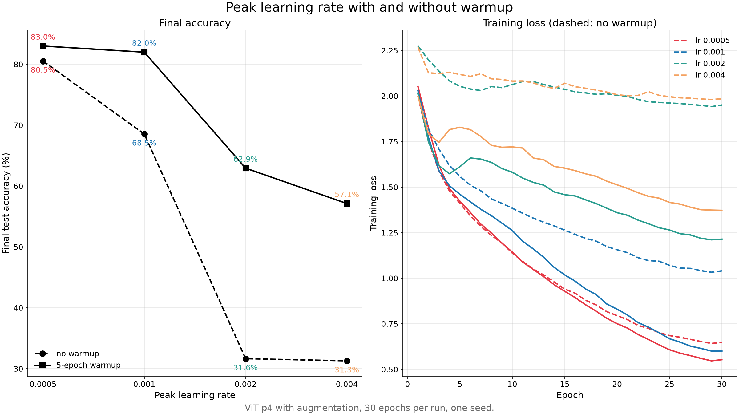
Warmup gave 11 points, so I looked at it more closely. I trained the patch-4 ViT at four peak learning rates, each with no warmup and with a 5-epoch warmup. Each run has 30 epochs and one seed.
| Peak learning rate | No warmup | 5-epoch warmup |
|---|---|---|
| 5e-4 | 80.5% | 83.0% |
| 1e-3 | 68.5% | 82.0% |
| 2e-3 | 31.6% | 62.9% |
| 4e-3 | 31.3% | 57.1% |
Warmup makes the model much less sensitive to the learning rate. At 5e-4, it adds 2.5 points. At 1e-3, it adds 13.5 points.
No run diverged to NaN. The runs with a high learning rate and no warmup stall instead: the training loss stays near 2.0 for all 30 epochs. For comparison, a model that guesses at random has a loss of about 2.3. So a run can fail without an error and still learn almost nothing.
Side study: less data
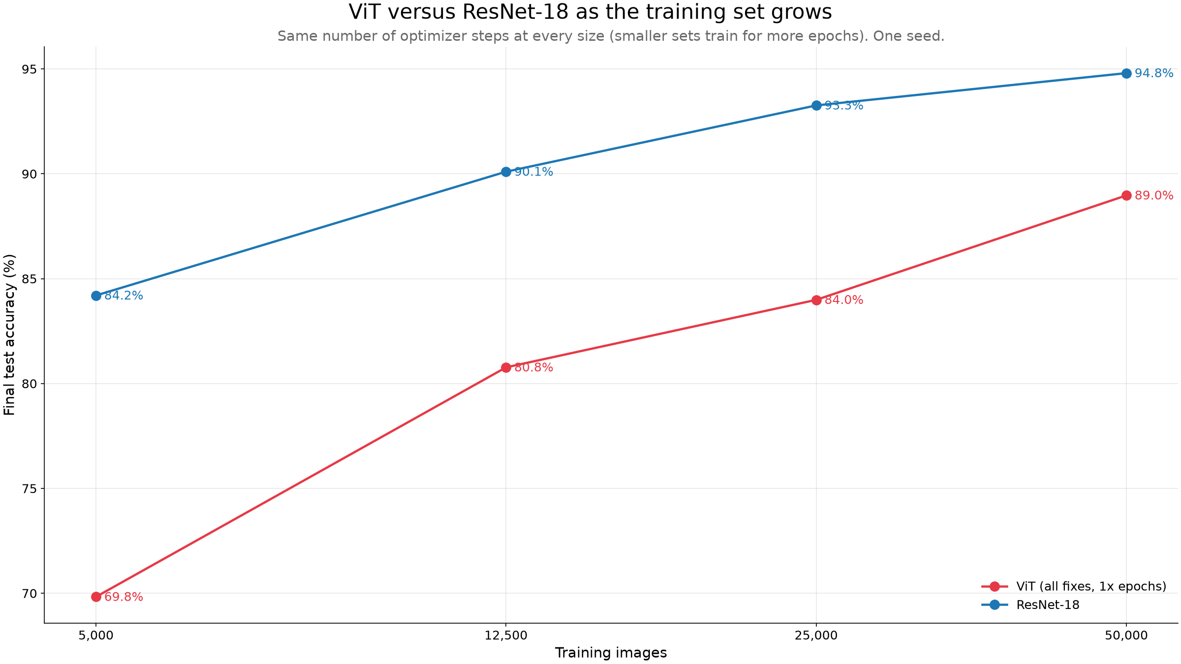
The second study trains the ViT (all fixes, 100 epochs) and ResNet-18 on 10%, 25%, 50% and 100% of the training set. Smaller sets train for more epochs, so every run takes the same number of optimizer steps. Each run uses one seed.
| Training images | ViT | ResNet-18 | Gap |
|---|---|---|---|
| 5,000 | 69.8% | 84.2% | 14.4 |
| 12,500 | 80.8% | 90.1% | 9.3 |
| 25,000 | 84.0% | 93.3% | 9.3 |
| 50,000 | 89.0% | 94.8% | 5.8 |
ResNet-18 leads at every size. The gap is largest with the least data, at 14.4 points, and smallest with all of the data, at 5.8 points. This is the cost of the missing built-in idea about nearby pixels. The ResNet gets that idea for free, but the ViT needs more images to learn it.
What I take from this
- For a small ViT on small images, set the patch size and the warmup first. Together, they gave 27 of the 36 points between the first ViT and the last one.
- Do not judge a regularizer on a short schedule. With MixUp/CutMix and stochastic depth, the model was still learning at epoch 100.
- On 50,000 images, a ResNet-18 is still the cheaper and better model.
The next post looks inside these models: what the attention heads look at.
I write about reinforcement learning, transformers, multi-agent systems, and the tools I build along the way.