Small Vision Transformers: What the Attention Heads Look At
A small ViT trained on CIFAR-10 learns local attention in layer 1 and global attention in the last layers. The fixes that raise accuracy make it more local.

On this page
In the first post, a small ViT went from 57% to 92.9% test accuracy on CIFAR-10 in eight steps. I argued there that a ViT starts with no idea that nearby pixels belong together, and that it must learn this from the data. I saved the weights of each step, so I can test that claim. This post opens those models and measures where each attention head looks.
The code is in the repo. The analysis takes less than a minute on the GPU.
How attention works
The ViT cuts each 32×32 image into 64 patches of 4×4 pixels and turns each patch into a vector called a token. It also adds one extra token, the CLS token, which holds no part of the image. After the last layer, the classifier reads only the CLS token to decide the class. So the CLS token must gather what it needs from the patches.
Attention is how tokens share information. In each layer, every token computes three vectors from itself:
- a query, which describes what the token is looking for,
- a key, which describes what the token contains,
- a value, which is the information that the token passes on.
To update one token, the model compares its query with the key of every token, including itself. A good match gives a high score. The model turns the scores into weights that are positive and add up to 1. These weights are the attention. The new token is the weighted average of all the values. An attention map shows these weights on the image, with bright patches for large weights.
A head is one complete set of queries, keys and values. Each layer has 6 heads that work side by side, so one layer can look in 6 different ways at once. One head can focus on the patches around a token while another head looks across the whole image. My ViT has 7 layers, numbered 0 to 6, so it has 42 heads in total.
Two numbers for each head
For every head, I measured two numbers and averaged them over the first 1,000 test images.
- Mean attention distance (Dosovitskiy et al., 2021). For one patch, I take the pixel distance from its center to the center of every other patch and weight each distance by the attention. A small value means that the head looks at its neighbors. If a patch attended to all 64 patches equally, the value would be 16.5 px, which is the average distance between two patch centers on the 8×8 grid.
- Entropy. This measures how widely the attention spreads. A low value means that the head puts almost all of its weight on a few tokens. A high value means that it spreads its weight over many tokens. The unit is the nat, which comes from the natural logarithm. Equal attention to all 65 tokens (64 patches plus CLS) gives the maximum, ln 65 = 4.17 nats.
The two numbers answer different questions, so I need both. The figure below shows three made-up heads for one patch, which is outlined in blue. The local head spreads its weight over the patches next to it. The second head is just as focused, and its entropy is even lower, but it looks at three patches far away. The third head looks everywhere equally. Distance alone cannot separate “focused but far” from “spread everywhere”, and entropy alone cannot separate “local” from “focused but far”.
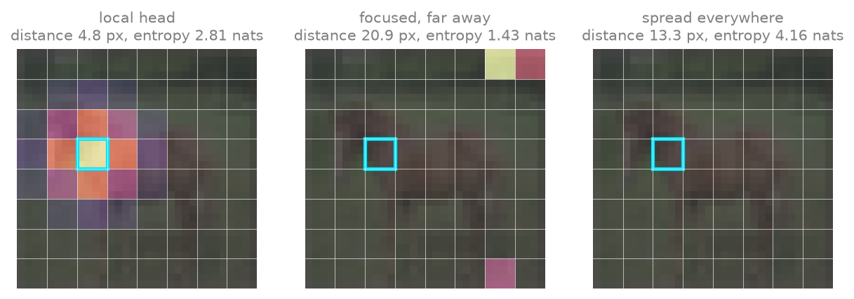
These examples use only the 64 patches, so their numbers differ a little from the real measurement, which also counts the CLS token. The uniform head shows 13.3 px instead of 16.5 px because this patch is near the center. Patches at the edges have more distant neighbors.
Local first, global later
The chart below is for the final ViT (all fixes, 200 epochs). Each dot is one head, and the line is the mean of the 6 heads in each layer.
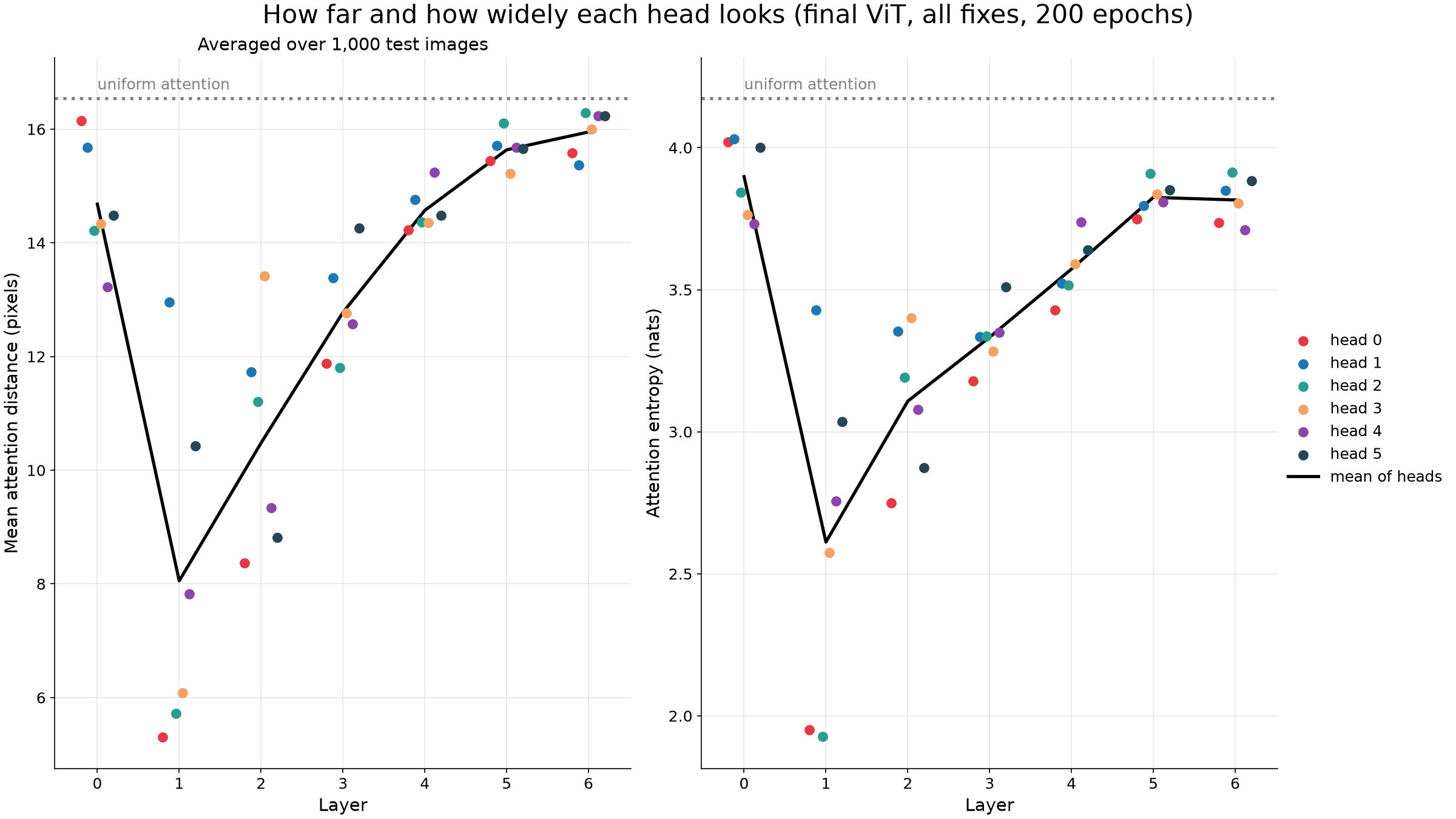
- In layer 0, the heads look almost everywhere. The mean distance is 14.7 px.
- In layer 1, the mean distance drops to 8.1 px. Three of the six heads look at patches about 5 to 6 px away. Since one patch is 4 px wide, these heads mostly look at the patches right next to the current one.
- From layer 2 to layer 6, the distance rises again until it is close to uniform (15.9 px).
The entropy has the same shape. It is lowest in layer 1 (2.6 nats) and highest in the last layers (3.8 nats).
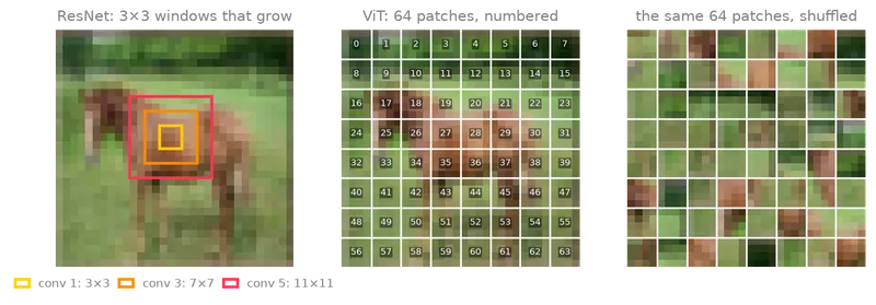
Nothing in the architecture asks for this. The ViT has no convolution, and it learns its position embeddings from random starting values. Still, it built a local stage that works like the small windows of a convolutional network, and it learned this stage from the data. The later layers then combine information from the whole image, much like the deep layers of a ResNet, whose view also covers the whole image.
Better models are more local
I ran the same measurement on every step of the ladder from the first post. This table shows the mean distance in layer 1. The patch-8 models have only 16 patches on a 4×4 grid, so their uniform value is a little different (16.1 px).
| Step | Test accuracy | Layer 1 mean distance |
|---|---|---|
| Patch 8, no augmentation | 57.3% | 15.8 px (uniform: 16.1) |
| + augmentation | 61.6% | 15.3 px (uniform: 16.1) |
| + patch 4 | 77.7% | 14.0 px |
| + warmup | 88.6% | 12.0 px |
| + label smoothing | 88.7% | 12.5 px |
| + MixUp/CutMix | 88.7% | 10.1 px |
| + stochastic depth | 88.3% | 9.6 px |
| + 2x epochs | 92.9% | 8.1 px |
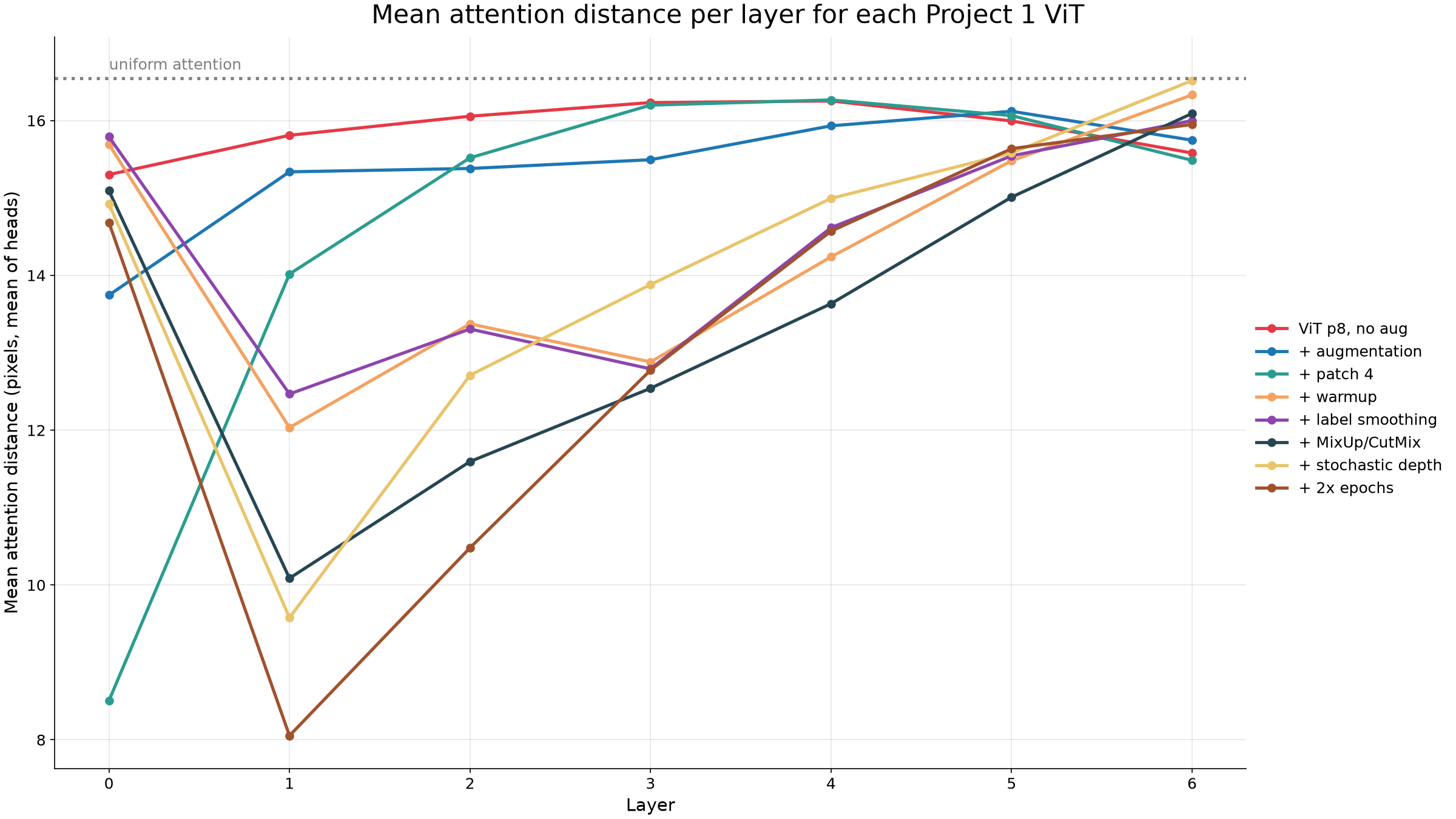
The chart shows three patterns:
- The two patch-8 models never become local. They stay close to uniform in every layer. Their entropy is low, so each patch focuses on a few patches, but those patches are not its neighbors. These models behave like the “focused but far” head in the example figure.
- Warmup moves the local stage. The patch-4 model without warmup has one local layer (layer 0, 8.5 px), and every later layer is close to uniform. With warmup, the local stage is in layers 1 to 3.
- The regularizers did change the model. In the first post, MixUp/CutMix and stochastic depth did not change the accuracy at 100 epochs. They did make layer 1 more local, from 12.5 px to 10.1 px and then 9.6 px. After 200 epochs, the model is the most local and the most accurate.
A caution: these are correlations from one checkpoint (seed 0) for each step. They do not show that local heads cause the higher accuracy.
One image, every head
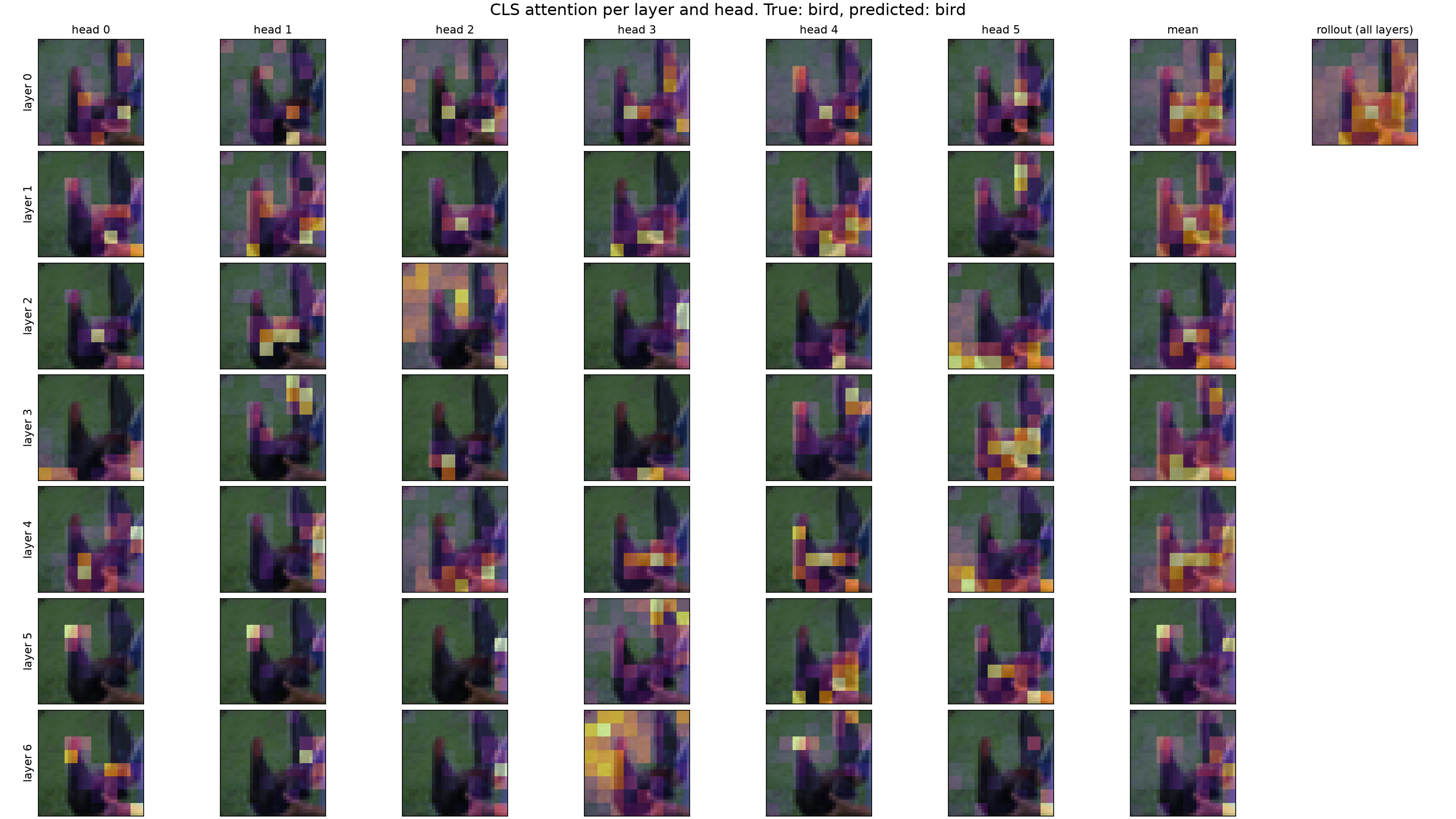
This grid shows how much the CLS token attends to each patch of one test image. The rows are layers and the columns are heads. The last two columns show the mean of the 6 heads and the attention rollout (Abnar and Zuidema, 2020). Rollout multiplies the attention maps of all layers together to estimate how much each input patch contributes to the CLS token at the end. It also accounts for the shortcut path around each attention layer.
A browser demo
The repo also has a small browser demo. You move the pointer over a patch, and the demo shows which patches that patch attends to, for each layer and head. Each map is scaled to its own maximum, so you should compare the shapes of the maps, not their brightness.
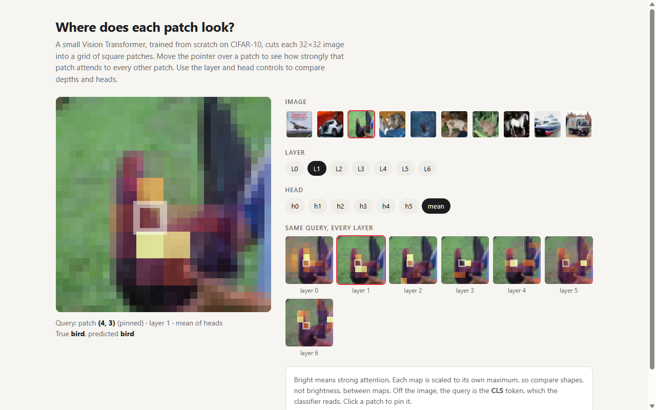
When I pin a patch on the bird in layer 1, it attends to the patches next to it. In layer 6, the same patch attends to a few patches across the image. This matches the numbers above.
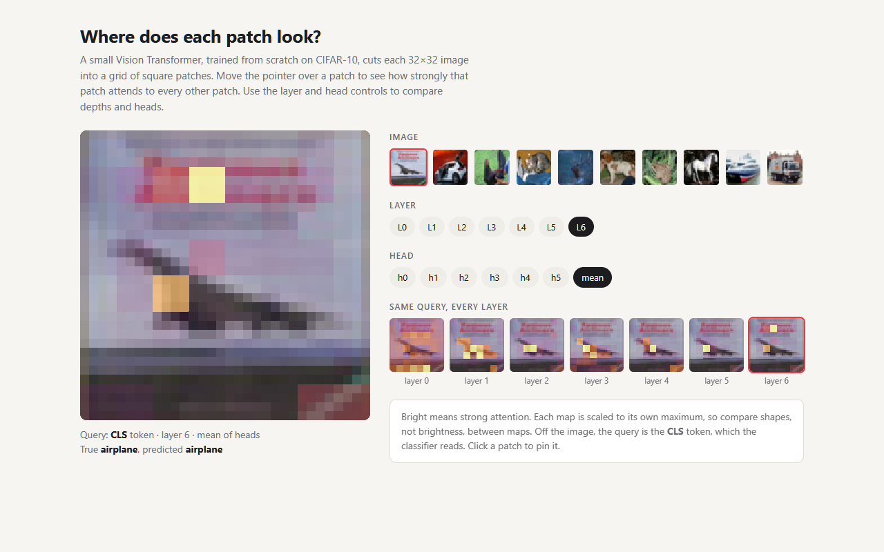
In the last layer, the CLS token of the airplane image attends to only a few patches. One is on the airplane, and the brightest one is on the sign behind it. A single image cannot show whether the CLS token usually picks the object.
The next post leaves CIFAR-10 and compares fine-tuning with training from scratch.
I write about reinforcement learning, transformers, multi-agent systems, and the tools I build along the way.