Small Vision Transformers: One-Step Images with MeanFlow
MeanFlow learns average velocities, so one model call makes an image: FID-10k 39.9 at NFE 1 and 17.5 at NFE 2. The first run diverged; here is why.

On this page
In the last post, flow matching needed 32 model calls to reach FID-10k 20.2. With one Euler step it gave a blurred average image. This post tries a method built for very few steps: MeanFlow (Geng et al., 2025).
The first run failed. The loss rose from 4 to above 10,000 in 14 epochs, and the samples were noise. The fix was one number. I’ll show both runs.
From velocity to average velocity
Flow matching learns the velocity v at one moment: the direction to move the image at time t. To go from noise to an image, a sampler adds up many small steps along v. One big step goes wrong, because the direction changes along the way.
MeanFlow learns the average velocity u over an interval, from time r to time t. If the model knows u, one step crosses the whole interval exactly:
With r = 0 and t = 1, that’s one step from pure noise to an image.
There’s no data for u directly, but there’s an identity that links it to v. The average velocity times the interval length is the integral of v. Take the derivative of both sides with respect to t, and you get the MeanFlow identity:
The training target is the right-hand side, with the gradient stopped. The derivative du/dt is the change of the model output when z and t move together along the path. It’s a Jacobian-vector product (JVP): one forward-mode pass through the network.
How I trained it
The DiT is the same as before, with one change. It gets a second time input, the interval length t − r, with its own embedding. That adds 131,584 parameters, for 9,937,420 in total.
- Times: r and t both come from a logit-normal distribution (mean −0.4, standard deviation 1). For 75% of each batch, r = t. Then the target is the plain velocity, which is flow matching.
- Guidance in the target: the target mixes the conditional and the unconditional velocity with scale 2. So the model learns the guided field, and sampling needs one call per step, not two.
- Loss weight: each sample’s squared error is divided by itself plus 0.001. This adaptive weight keeps a few huge errors from taking over a batch.
- JVP: I compute it with
torch.func.jvpand no gradient, since the target is stopped anyway. The fused attention kernels in PyTorch have no forward-mode derivative, so the JVP runs with the plain math attention.
The rest is the same as for DDPM and flow matching: same data, optimizer, EMA and 200 epochs.
The first run: time scale 1000
The DiT’s timestep embedding was built for DDPM, with timesteps from 0 to 999. So for flow matching I multiply t by 1000 before the embedding. I did the same for MeanFlow, and training diverged.
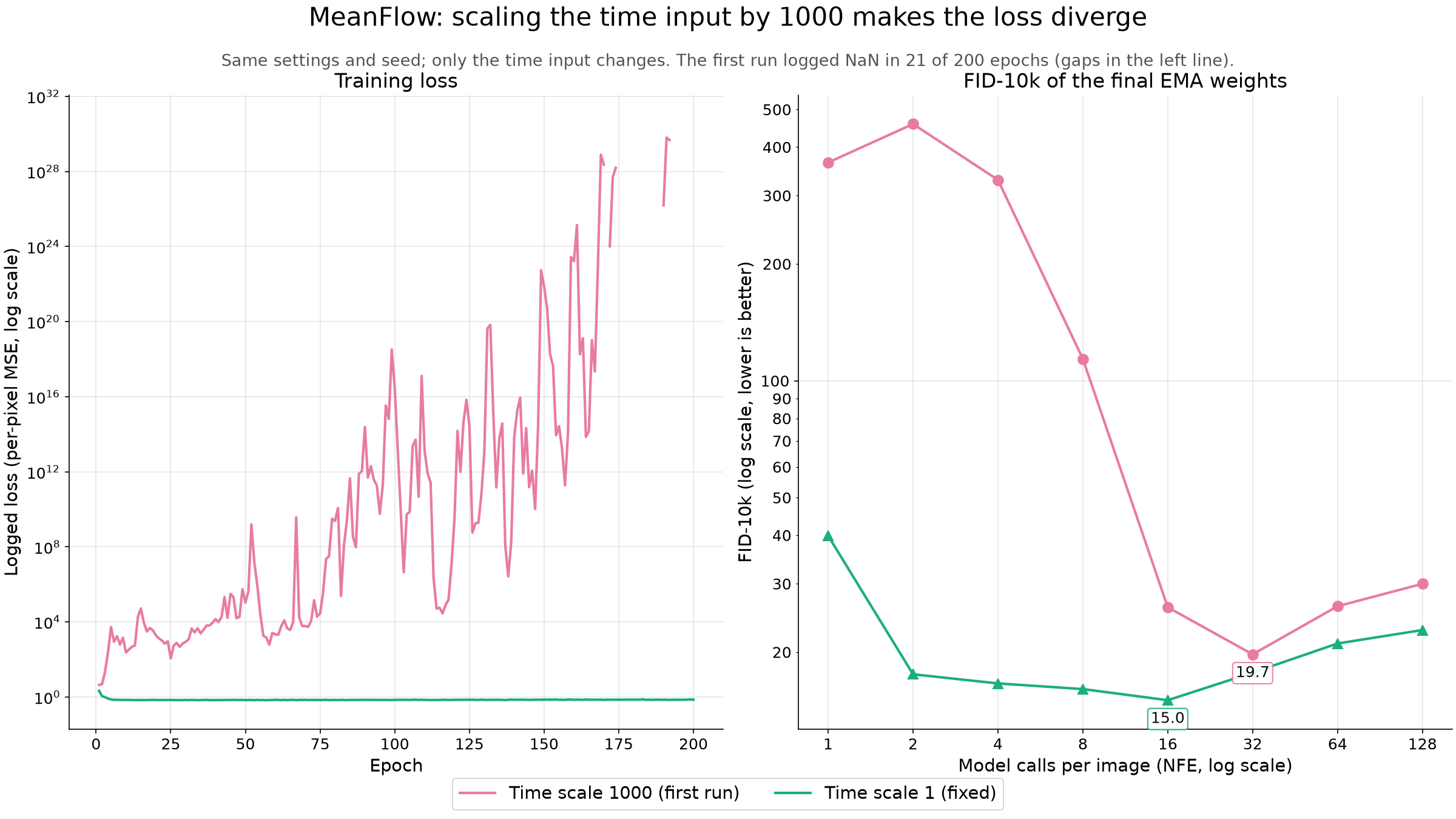
With time scale 1000, the logged loss went from 4.4 in epoch 1 to 5,316 in epoch 5 and 18,884 in epoch 14. The largest finite value was 3.4 × 10^30. In 21 of the 200 epochs, starting at epoch 171, the logged loss was NaN.
Here’s my reading of why. The target contains du/dt, and that includes the derivative of the model output with respect to t. The sinusoidal time embedding computes sin(1000 · t · ω). Its derivative with respect to t has a factor of 1000. So du/dt, and with it the target, can be about 1000 times larger than it should be. The target comes from the model itself, so a larger output gives a larger target, which pushes the output larger again.
The fix was to give the DiT the raw times in [0, 1], with no scale, as the paper does. Nothing else changed. With time scale 1, the loss falls from 2.15 in epoch 1 and stays flat (0.72 in epoch 200).
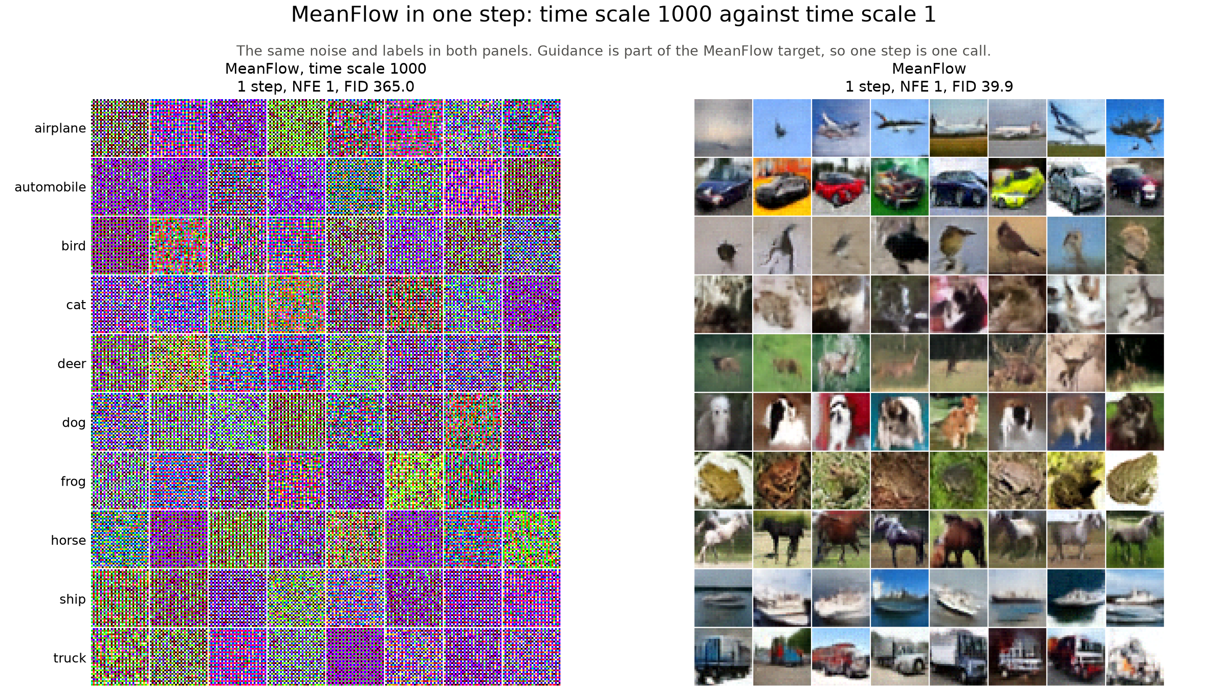
One thing surprised me. The broken run still had usable weights at the end: FID-10k 19.7 with 32 steps. My guess is that gradient clipping (norm 1) and the adaptive weight kept each update small, so the huge loss values didn’t reach the weights. I didn’t check this. Either way, the broken run was useless at the job it was trained for: with one step, its FID was 365.0.
Results with the fix
| NFE (steps) | MeanFlow FID-10k |
|---|---|
| 1 | 39.9 |
| 2 | 17.5 |
| 4 | 16.6 |
| 8 | 16.1 |
| 16 | 15.0 |
| 32 | 17.7 |
| 64 | 21.0 |
| 128 | 22.8 |
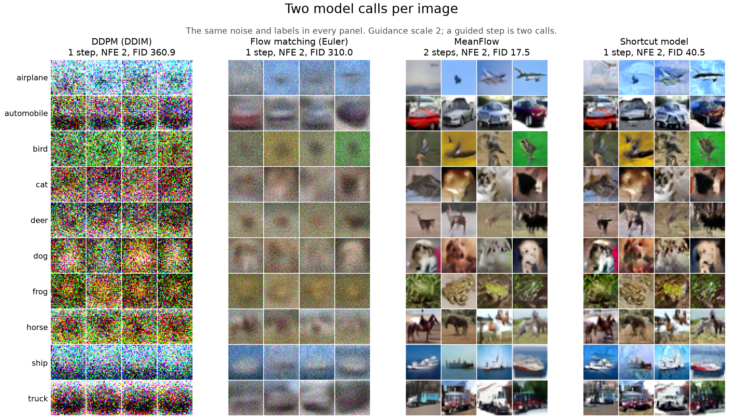
One model call gives FID 39.9. Two calls give 17.5. For comparison, flow matching needed 64 Euler calls to get to 16.5 and gave 310.0 with 2 calls.
FID gets worse after 16 steps: 22.8 with 128 steps. I didn’t find out why. The method is built for few steps, and 75% of its training is at r = t, so I’m not surprised that many tiny steps aren’t its strength. That’s a guess, not a test.
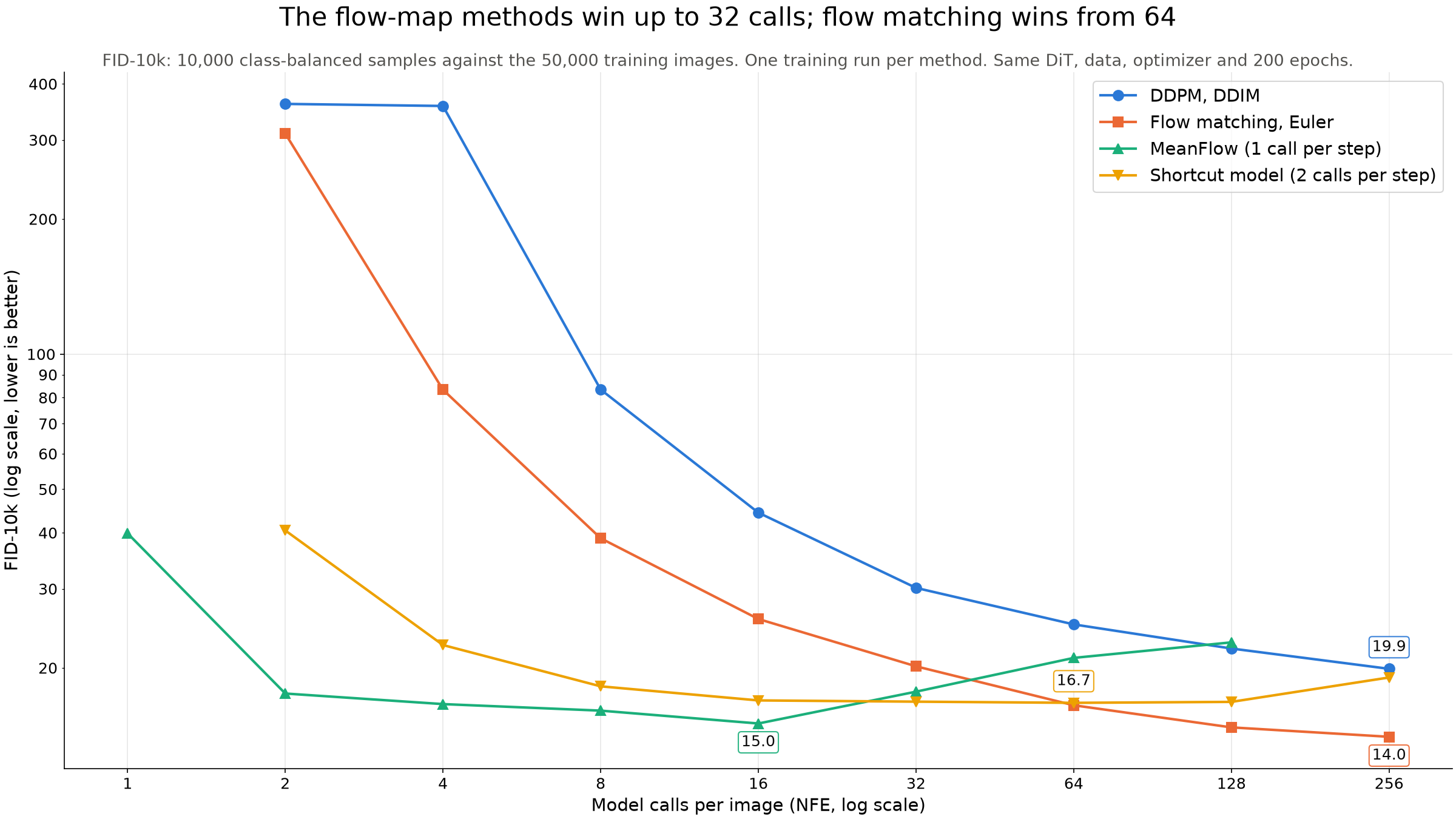
The chart also has the shortcut model, the subject of the next post. At two model calls per image, the difference between the methods is easy to see:
The cost
MeanFlow isn’t free. The JVP and the extra unconditional pass for the guided target make each epoch about twice as slow.
| Flow matching | MeanFlow | |
|---|---|---|
| Time per epoch | 25.9 s | 50.5 s |
| Training time (200 epochs) | 86.2 min | 168.4 min |
| Peak VRAM | 3,595 MiB | 3,599 MiB |
Both trained for the same 200 epochs, so MeanFlow saw the same data but used twice the compute. I didn’t train flow matching for 400 epochs to match the compute.
Limits
- I trained each setting once, with one seed, so I can’t say how much FID changes from one seed to another.
- I computed FID from 10,000 samples (FID-10k). FID from fewer samples is biased upward, so these values are higher than the FID-50k (50,000 samples) that papers report. Compare them with each other, not with published results.
- The two MeanFlow runs differ only in the time scale, but each has one seed, so I can’t separate the effect of the fix from run-to-run noise at 32 steps. At 1 to 4 steps, the gap (365.0 against 39.9 at one step) is far too large to be noise.
- MeanFlow used about twice the training compute of flow matching for the same 200 epochs. I didn’t train flow matching longer to match it.
Run it
- Train MeanFlow. The time scale of 1 is the default in
tinydit/constants.py. - Compute FID-10k for 1 to 128 steps.
uv run python scripts/train_diffusion.py --method meanflow
uv run python scripts/evaluate_fid.py --method meanflow --steps 1 2 4 8 16 32 64 128
The code is in the repo.
What I take from this
- A 9.9 M parameter DiT makes recognizable CIFAR-10 images in one model call with MeanFlow, and two calls get it to FID-10k 17.5.
- If the target contains a derivative of the model, check every scale factor on the inputs. A factor of 1000 on t became a factor of 1000 in the target.
- The extra JVP costs about twice the training time per epoch.
I write about reinforcement learning, transformers, multi-agent systems, and the tools I build along the way.