Small Vision Transformers: Diffusion Models as Image Classifiers
A diffusion model that was never trained to classify gets 86.7% on CIFAR-10 with 1,000 calls. A joint image and label model gets 87.2% with one call.

On this page
- A diffusion model is already a classifier
- The first result looked wrong
- Normalizing the levels
- Which noise levels know the class?
- Where it goes wrong
- A model that learns images and labels together
- The joint model classifies in one call
- But its images are worse
- Two ways to make it better
- Limits
- Run it
- What I take from this
Every diffusion model in this series so far took a class label and drew an image. This post turns that around: can the same models tell me the class of an image?
I try two ways. The first uses the trained DDPM and flow-matching models from the earlier posts as they are, with no new training. The second trains a new model that learns images and labels together, so it can go in both directions.
A diffusion model is already a classifier
A class-conditional diffusion model learns to remove noise from an image when it knows the class. If I give it the wrong class, it removes the noise less well. That’s the whole idea of the diffusion classifier (Li et al., 2023):
- Add noise to a test image.
- Ask the model to remove the noise once for each of the 10 classes.
- Predict the class with the lowest error.
One noise sample is noisy, so I repeat this at 100 noise levels and average. At each level, all 10 classes see the exact same noise, so the only thing that changes between them is the label.
The cost is high. Each level needs 10 model calls (one per class), so 100 levels cost 1,000 DiT calls per image. A trained classifier needs one.
I store every error in a table: 10,000 test images × 10 classes × 100 levels. Then every way of combining the levels is a cheap calculation on the table, with no new GPU pass. Building one table took about 25 minutes on one RTX 3080 Ti.
The first result looked wrong
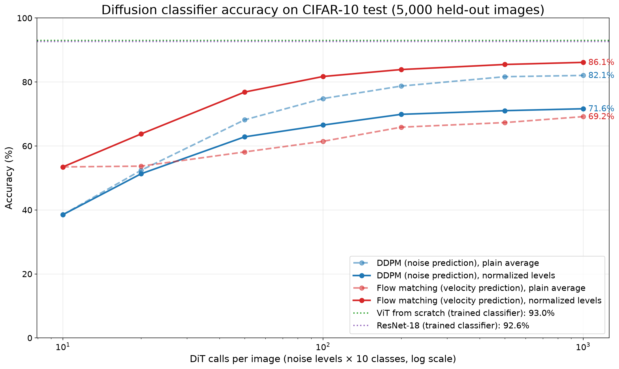
With a plain average over all 100 levels, the DDPM model gets 82.1% and the flow-matching model gets only 69.2%. That surprised me, because flow matching made better images in every earlier post.
The reason is the scale of the errors. Only the difference between the 10 class errors matters for the vote, so I measured how much the class errors differ at each level:
- Flow matching: the model predicts a velocity, and the difference between classes grows about 15 times from the least noise to the most noise. In a plain average, the noisiest levels decide the vote, and those levels say the least about the class.
- DDPM: the model predicts the noise, and the difference between classes is largest at little and medium noise. At high noise it’s close to zero. So a plain average already listens most to the useful levels.
Normalizing the levels
The fix is to put every level on the same scale. For each level, I take the errors of the 10 classes, subtract their mean, and divide by the typical spread between classes at that level. After that, every level gets about the same say.
To keep the test honest, I split the 10,000 test images in two. I fit every choice (the scales, a window of levels, and a set of learned weights) on the first 5,000 images and report accuracy on the other 5,000.
| Scoring (5,000 held-out images, 1,000 calls) | DDPM | Flow matching |
|---|---|---|
| Plain average of all levels | 82.1% | 69.2% |
| Best window of levels | 82.1% | 84.1% |
| Normalized levels | 71.6% | 86.1% |
| Best window of normalized levels | 80.4% | 86.7% |
| 100 learned level weights | 82.4% | 86.6% |
With normalized levels, flow matching wins: 86.7% against 82.4% for the best DDPM scoring. Normalization hurts DDPM, though, from 82.1% to 71.6%. DDPM’s noisy levels had almost no say before, and they’re weak. Normalization gives them the same say as the good levels.
The learned weights (one per level, fitted with logistic regression) add almost nothing over the simpler methods. So for these models, the right scale per level is most of what a weighting can do.
For comparison, the ViT from the first post gets 93.0% and the ResNet-18 judge from the DDRL post gets 92.6%, each with one call. So the diffusion classifier is 6 points behind, at 1,000 times the cost.
Which noise levels know the class?
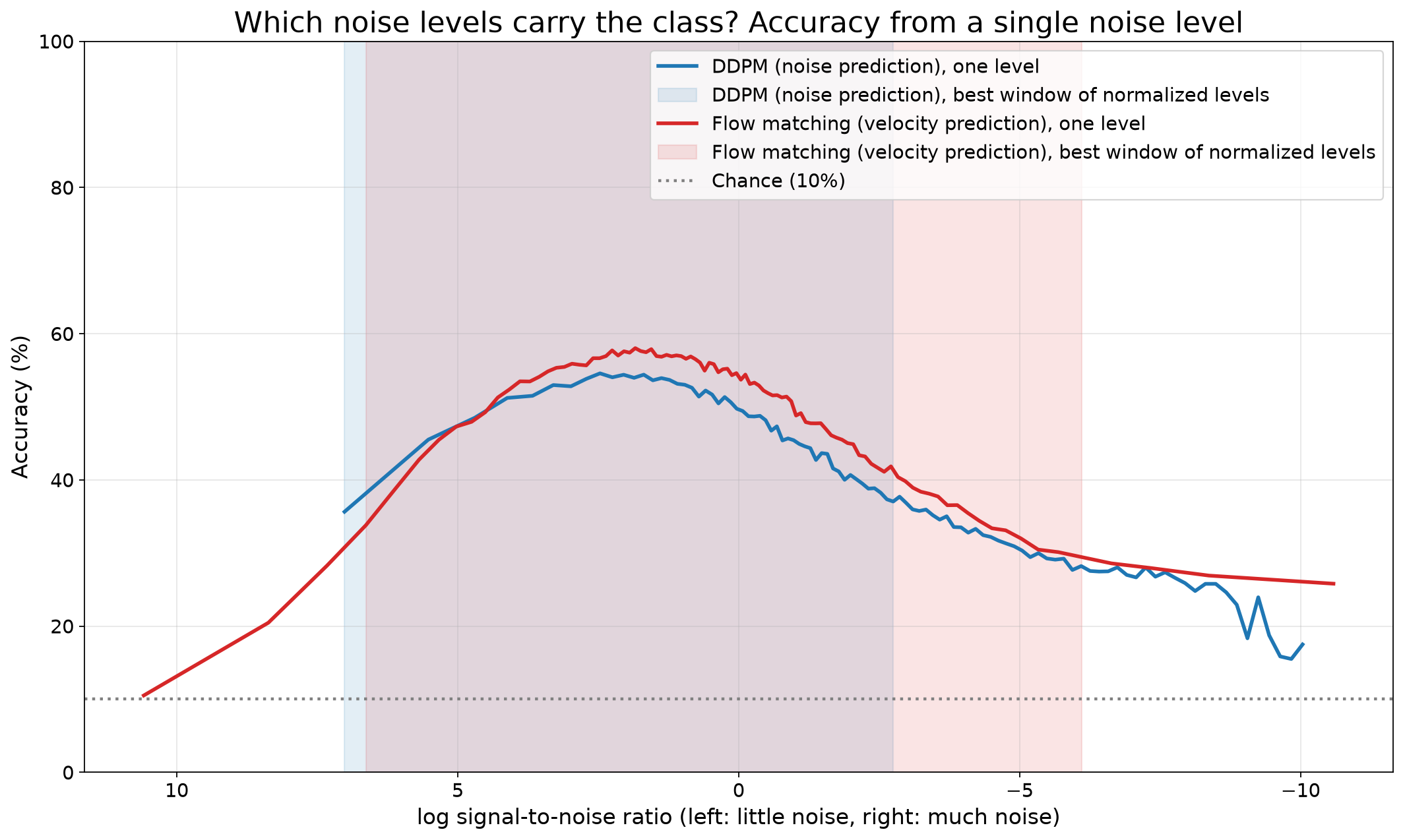
One level alone gives at most 58% (flow matching) or 55% (DDPM), near a log signal-to-noise ratio of 2. That’s the middle of the noise range.
At the two ends, the label stops mattering:
- Little noise: there’s almost nothing to remove, and the model can do it from the image alone. Flow matching at its cleanest level is at chance (10%).
- Large noise: the image is almost gone, so I think the model can only guess a typical image of each class, and the test image has little effect on the result.
Flow matching is more accurate than DDPM at every level from log SNR 4.5 to the noisiest. With less noise than that, DDPM is more accurate.
I also checked the precision. On 500 test images, bfloat16 and float32 give the same prediction for 99.0% of them, so I built the tables in bfloat16.
Where it goes wrong
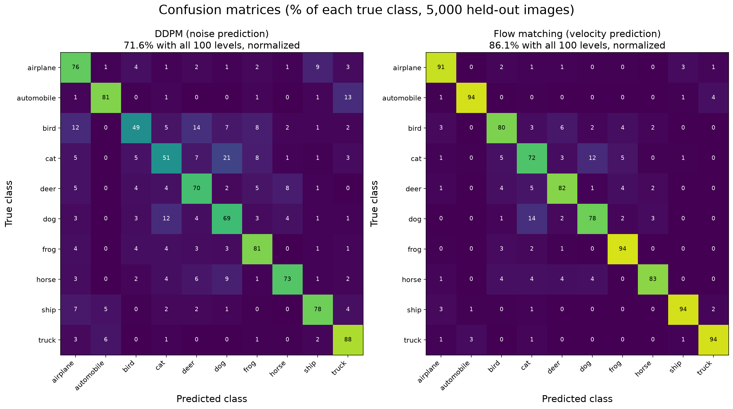
Cats and dogs get mixed up most. With DDPM, 21% of the cats go to dog. Bird, cat and dog are the weakest classes for both models, and the vehicles and frog are the strongest.
A model that learns images and labels together
The diffusion classifier works, but 1,000 calls per image is a lot. So I trained a second kind of model: one network that treats the image and the label as two things to denoise, in the style of UniDiffuser (Bao et al., 2023).
- The label is a vector too. It has +1 for the class and −1 for the other nine. The DiT gets it as one extra token next to the image patches.
- Two noise levels. The image and the label each get their own time, and both condition every block. The model predicts a flow-matching velocity for each.
- Four training modes. Each training example draws one:
- Generate (40%): the label is clean, so the model learns to draw an image for a label.
- Classify (30%): the image is clean, so the model learns to find the label of an image.
- Unconditional (10%): the label is pure noise, for classifier-free guidance.
- Independent (20%): both are noisy at independent levels.
Everything else is the same as the flow-matching model from earlier: the same DiT size (9.9 M parameters with the label token), AdamW at 3e-4, batch 128, 200 epochs and an EMA with decay 0.9999. Training took 88 minutes on one RTX 3080 Ti.
To classify, I keep the image clean and run Euler steps on the label, starting from noise. Each step is one DiT call. The predicted class is the largest entry of the final label vector.
To generate, I keep the label clean and run Euler steps on the image with guidance of scale 2. Each guided step is two calls.
The joint model classifies in one call
| Label steps (DiT calls) | 1 | 2 | 4 | 8 | 16 | 32 |
|---|---|---|---|---|---|---|
| Accuracy (10,000 test images) | 85.9% | 84.6% | 83.3% | 82.8% | 82.4% | 82.3% |
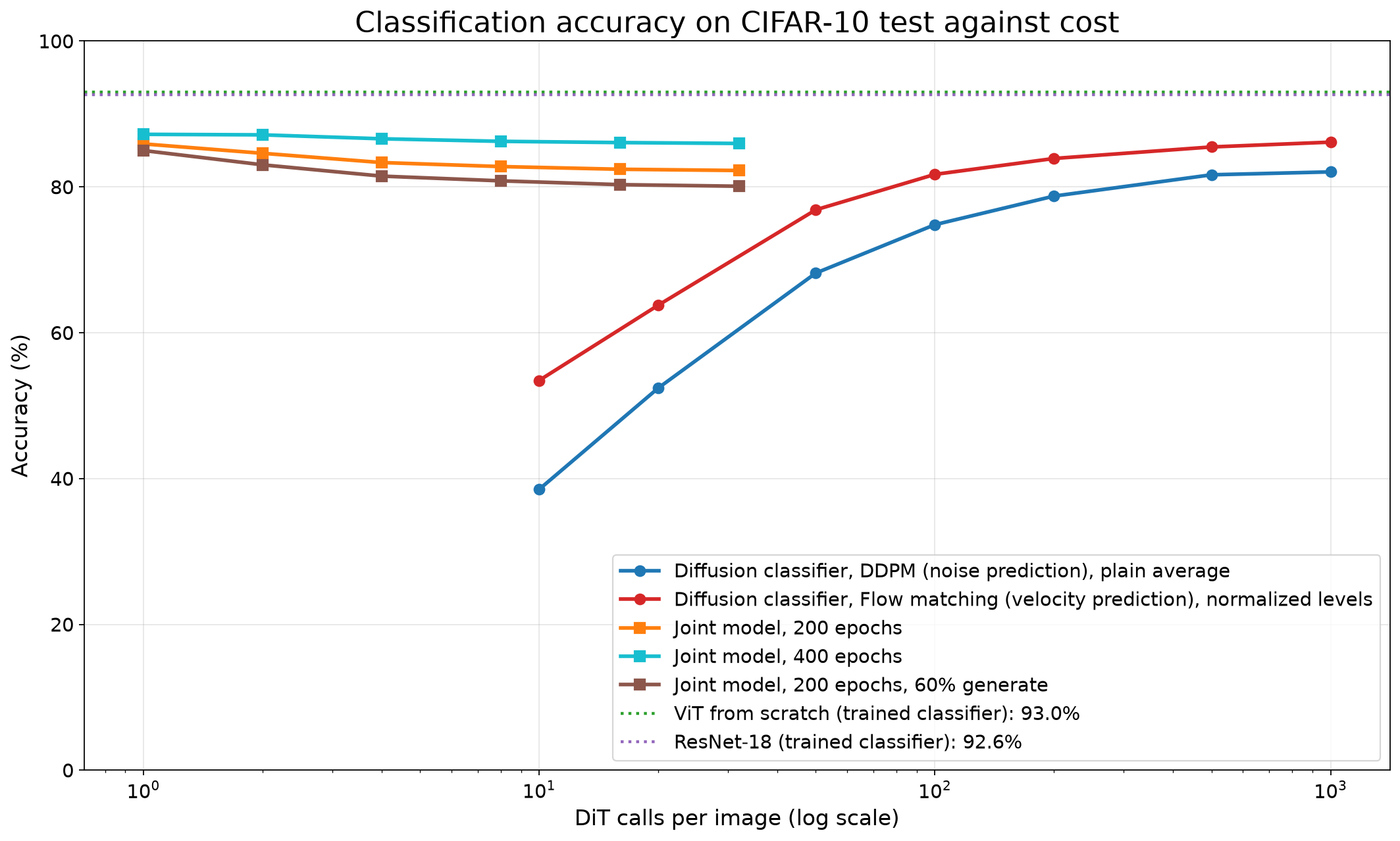
With a single call, the joint model gets 85.9%. That’s almost the 86.7% of the best diffusion classifier, which needs 1,000 calls.
More steps make it worse. I think the reason is that one step from pure noise gives the model’s best guess of the clean label directly, which is all a classifier needs. Each extra step starts from a noisier mix of the guess and the random start, and adds a little of that randomness.
But its images are worse
| Image steps (DiT calls) | 16 (32) | 64 (128) | 128 (256) |
|---|---|---|---|
| Joint model, FID-10k | 51.8 | 50.9 | 53.2 |
| Flow-matching DiT from the earlier post | 20.2 | 14.7 | 14.0 |
The same training budget gives much worse images. Too much guidance can make FID worse, so I tried other scales at 64 steps:
| Guidance scale | 1.0 | 1.5 | 2.0 | 3.0 |
|---|---|---|---|---|
| FID-10k | 57.1 | 53.3 | 50.9 | 50.9 |
The guidance isn’t the problem.
Two ways to make it better
I had two guesses. First, the model was still learning: its quick test accuracy rose every time I checked, up to epoch 200. Second, only 40% of the training examples teach it to draw an image for a label, against 100% for the image-only model. So I ran two more:
- 400 epochs: the same run, trained 200 epochs more with the same settings.
- 60% generate: a new 200-epoch run with more generation examples. The shares are 60% generate, 20% classify, 10% unconditional and 10% independent.
| Label steps (DiT calls) | 1 | 2 | 4 | 8 | 16 | 32 |
|---|---|---|---|---|---|---|
| 200 epochs | 85.9% | 84.6% | 83.3% | 82.8% | 82.4% | 82.3% |
| 400 epochs | 87.2% | 87.1% | 86.6% | 86.3% | 86.1% | 86.0% |
| 200 epochs, 60% generate | 85.0% | 83.0% | 81.5% | 80.8% | 80.3% | 80.1% |
| Image steps (DiT calls), FID-10k | 16 (32) | 64 (128) | 128 (256) |
|---|---|---|---|
| 200 epochs | 51.8 | 50.9 | 53.2 |
| 400 epochs | 41.5 | 39.3 | 39.0 |
| 200 epochs, 60% generate | 40.9 | 38.6 | 39.6 |
| Flow-matching DiT (200 epochs) | 20.2 | 14.7 | 14.0 |
Both helped the images by about the same amount: FID at 64 steps went from 50.9 to 39.3 with more epochs, and to 38.6 with more generation examples. But they cost different things:
- More epochs cost twice the training time and improved the classifier too. At 87.2% with one call, it now beats the 86.7% of the best diffusion classifier with 1,000 calls. (That number comes from the 5,000 held-out images, and this one from all 10,000, so it’s a close call, not a clear win.)
- More generation examples cost nothing in time, but the classifier lost 0.9 points.
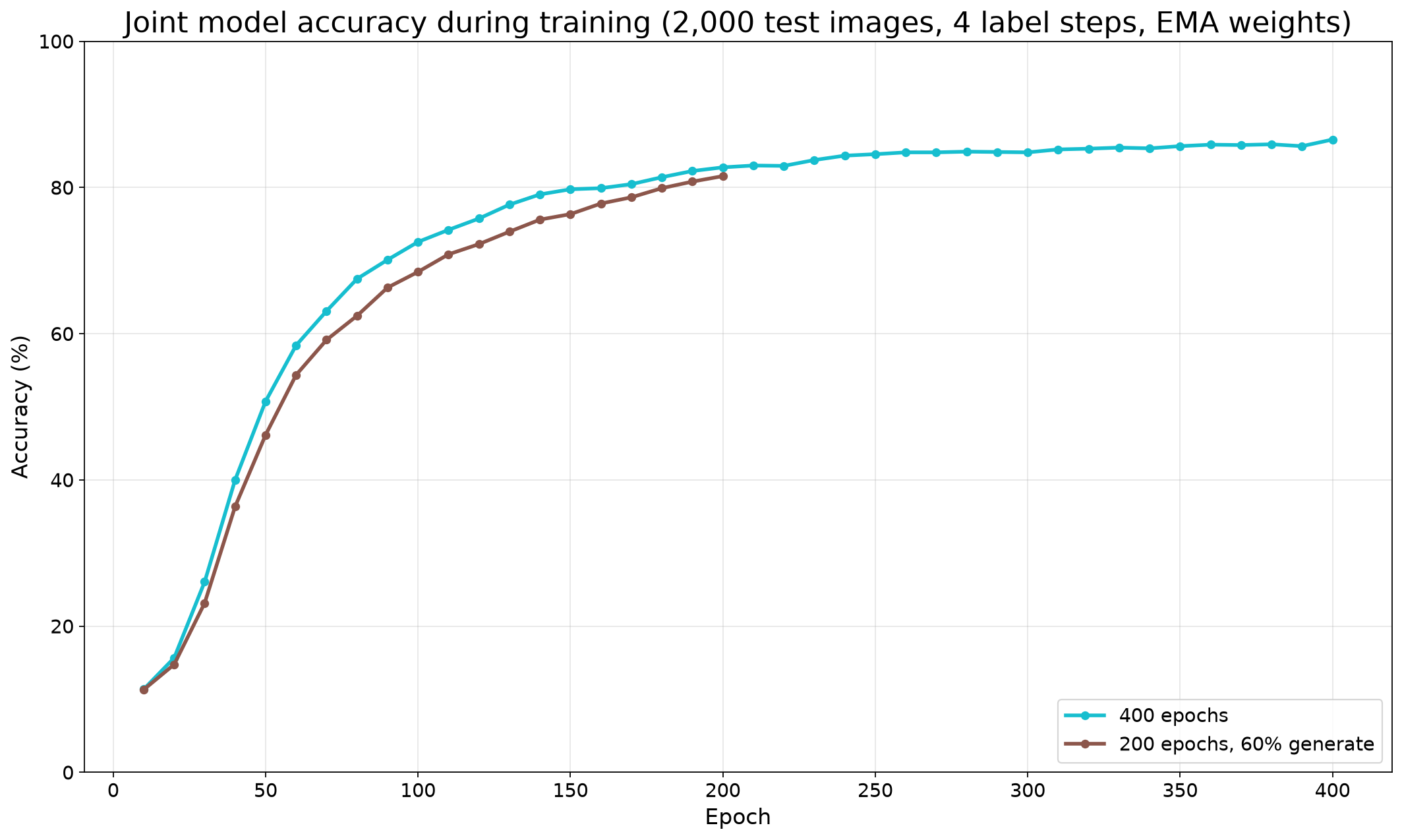
The accuracy curve flattens after about epoch 250, so more epochs alone won’t close the gap to the trained classifiers at 93%.
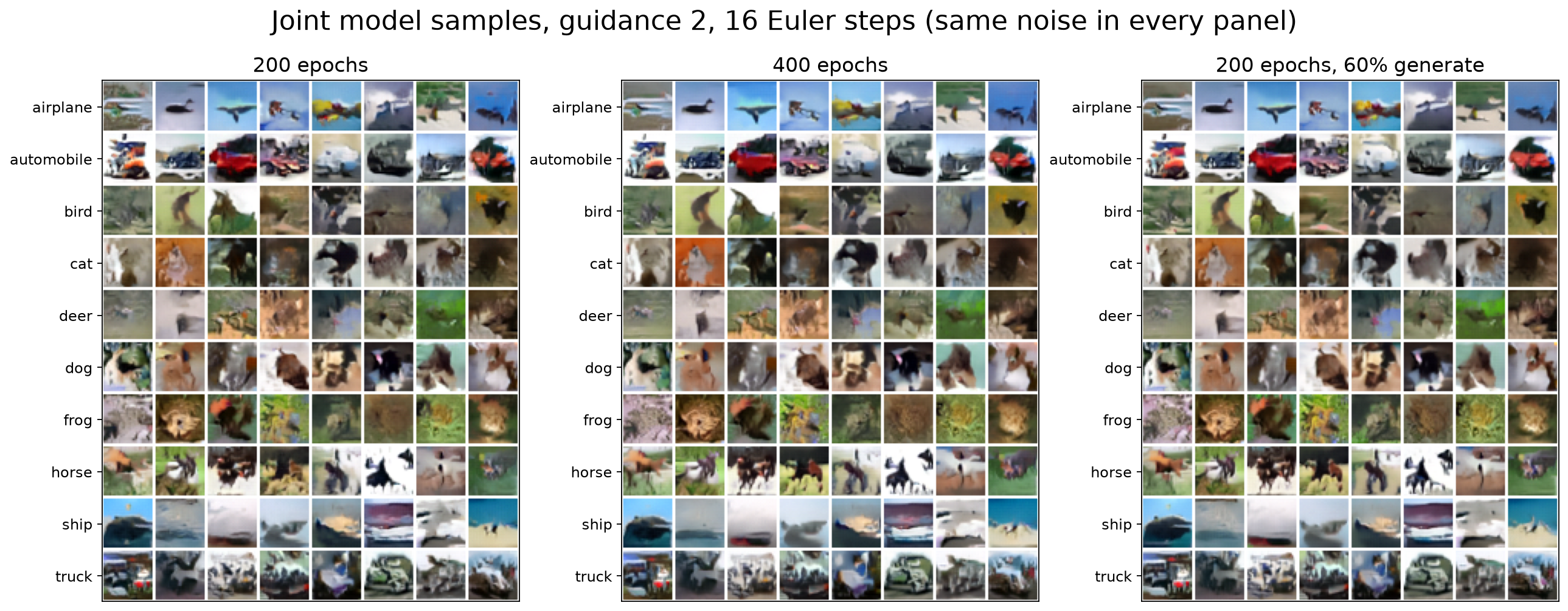
The same noise gives the same layout and colors in all three models. The later models draw slightly cleaner shapes, but the gap to the image-only model is still large: FID 38.6 at best, against 14.7. My two guesses explain only part of it, and I don’t know the rest yet.
Limits
- I trained each model once, with one seed, so the 0.5-point gap between the joint model and the diffusion classifier could change with another seed.
- I fit the level choices on half of the test set and report on the other half. The two halves come from the same test set, so the held-out numbers are fair, but they come from only 5,000 images.
- The diffusion classifier uses 100 noise levels with one noise sample each. More samples per level could change the numbers.
- I computed FID from 10,000 samples (FID-10k). FID from fewer samples is biased upward, so these values are higher than the FID-50k (50,000 samples) that papers report. Compare them with each other, not with published results.
Run it
- Copy the trained DiT weights from a local clone of tiny-diffusion-transformer.
- Build the error table for each model.
- Compute the accuracies and draw the figures.
- Train and evaluate the joint model.
- Train and evaluate the joint model with 60% generation examples.
uv run python scripts/import_checkpoints.py
uv run python scripts/compute_errors.py --method ddpm
uv run python scripts/compute_errors.py --method flow_matching
uv run python scripts/analyze.py --baseline "ViT from scratch=0.9302" --baseline "ResNet-18=0.9261"
uv run python scripts/train_joint.py
uv run python scripts/evaluate_joint.py
uv run python scripts/train_joint.py --run-name joint_gen60 --mode-shares 0.6 0.2 0.1 0.1
uv run python scripts/evaluate_joint.py --run-name joint_gen60
The code is in the repo.
What I take from this
- A class-conditional diffusion model is a classifier for free, but only if I weight its noise levels with care. For the flow-matching model, a plain average gave 69.2%, and a per-level scale gave 86.7%.
- The diffusion classifier is slow (1,000 calls) and still 6 points behind a ViT trained to classify.
- A model that learns images and labels together classifies just as well with one call, and its accuracy kept rising with training.
- The price is image quality. On the same small DiT, the joint model’s best FID is 38.6, against 14.7 for the image-only model.
I write about reinforcement learning, transformers, multi-agent systems, and the tools I build along the way.